当前位置:网站首页>Paper reading - joint beat and downbeat tracking with recurrent neural networks
Paper reading - joint beat and downbeat tracking with recurrent neural networks
2022-06-13 02:15:00 【zjuPeco】
List of articles
1 summary
Recently, I have been working on projects related to music cards , Need to understand the basic characteristics of music , such as beats and downbeats Is the most basic feature .madmom It's a pair I found beats and downbeats Third party libraries are available for the detection of , So I studied hard , Write down the methods used and your understanding .
madmom Medium beats and downbeats The test is a recurrence Joint Beat and Downbeat Tracking with Recurrent Neural Networks This paper , The core idea is HMM, If the HMM Without a solid understanding , I suggest you read another article I wrote first understand HMM. This article will not HMM The basic concept of .
Before speaking about the thesis , Let me first explain some special terms in music , Align some concepts , It is convenient for the following narration . Some terms may not reappear in this article , But it helps to understand music , It was written together .
| Noun | A term is used to explain |
|---|---|
| time (beat) | In music , Time is divided into equal basic units , Each unit is called a “ time ” Or one shot . |
| Strong shot (downbeat) | A strong beat in music . yes beats Subset . It is usually the beginning of each section beat |
| Section (measure/bar) | Music is alternating between strong and weak beats , It is to organize a section according to a certain law to form the smallest beat , And then cycle back and forth on this basis . A section usually has 2 pat ,3 pat ,4 Shoot or 6 Shoot and wait |
| Rhythm (meter) | beats per measure, The beat of a song , It is generally expressed as 1/4 Shoot or 2/4 Shoot or 3/8 Shoot and wait . such as 3/4 Beat representation 4 It's divided into 1 pat , Each section has 3 pat , The beat intensity is strong 、 weak 、 weak . |
| Global rhythm (tempo) | It's usually used bpm(beats per minute) To make the unit , Indicates how many... Are there per minute beats, To measure the speed of music , A piece of music can be composed of different tempo play . |
| Local rhythm (tempi) | Every two adjacent beats There can be differences between 1/16 note , or 1/8 note , or 1/4 And so on , This is the local rhythm |
| onset | The moment when a note is sounded by an instrument or a person . |
| Peak value (peak) | onset The peak of the envelope , concrete peak_pick. |
Back to this paper . In a nutshell, this paper is to cut the signal into several frames, Every frame Will be in RNN After the network corresponds to a probability output , It means that we should frame yes beat still downbeat Still not .HMM We will use this to calculate the launch probability RNN result , hold frame stay measure The relative position and tempi As an implicit variable , Get the best hidden variable path , And decode the path into beats and downbeats.
Each step will be explained step by step below , The point is HMM And the prediction part . These two parts are a bit confusing .
2 Signal preprocessing
This part is actually a similar to MFCC The process of extracting speech signal features , As RNN The input of , Here is a brief introduction . First, the Hanning window is used to segment the signals with overlap , Divided into 100fps(frame per second), Based on this, the short-time Fourier transform (STFT). The phase feature is discarded , Only amplitude features are preserved , Because the human ear cannot recognize the phase . In order to ensure the accuracy of time domain and frequency domain , do STFT when , Used separately 1024,2048 and 4096 Three window sizes . Limit the frequency band to [30, 17000]Hz The scope of , And give each Octave. Divide up 3,6 and 12 Frequency bands , Corresponding to 1024,2048 and 4096 Three window sizes . At the same time, the first-order difference of the spectrum is also carried out , Also as a feature concat go in . Final , The characteristic dimension of the input network is 314.
3 Classification neural network
This part uses LSTM A network built by , The aim is to give each frame To classify , Output two probability values ,( yes beat Probability , yes downbeat Probability ), Take the larger as the frame The classification of . To avoid confusion ,downbeat Do not belong to beat.
meanwhile , Also set up θ = 0.05 \theta=0.05 θ=0.05 The threshold of , Only greater than this threshold , Will be judged as beat perhaps downbeat. This is to reduce the interference of blank space at the beginning and end of the music .
Since each frame yes beat still downbeat We know the probability of , Then I'll take each one directly frame Category of maximum probability , If both probabilities are relatively small, it is considered that it is neither beat Neither downbeat, This is what happened ?
The ideal is very good , This is not the case , Don't be misled by the pictures in the paper , Let's see what the actual output of the model looks like .
The output of the model is shown in the figure above 3-1 Shown , This is a 30s Left and right actual examples . The upper half of the graph is for each frame by beat Probability , The lower half of the graph is for each frame by downbeat Probability . Just look at downbeat In this part , It is not difficult to see that the probability is high frame The distance between them is long and short , And in a section (bar) among , Strong shot (downbeat) It should only appear once , The appearance of the second strong beat will interfere with it .RNN I don't know that the emergence of strong beat is periodic , So we need to HMM To determine which position is a strong shot , Which positions are weak shots , Where is nothing .
Think about it from another angle ,RNN I don't know music here meter How many shots , Without this information , want RNN It is very difficult to judge the strong beat and weak beat directly . Next section HMM Is the basis RNN Result , To choose the best beats and downbeats.
4 Dynamic Bayesian network (HMM)
This is the key part , Let's go into detail .Joint Beat and Downbeat Tracking with Recurrent Neural Networks The explanation of this part is not clear , Let's look directly at what it uses An Efficient State-Space Model for Joint Tempo and Meter Tracking As described in .
4.1 The original bar pointer model
As early as 2006 In the year ,Bayesian Modelling of Temporal Structure in Musical Audio I have proposed to use HMM solve beat tracking The way of the problem . Now the way , It is optimized on the basis of it , Let's take a look at the earliest version HMM How it was designed .
Let's make No k k k individual frame The implicit variable of is x k = [ Φ k , Φ ˙ k ] \bold{x}_k=[\Phi_k, \dot{\Phi}_k] xk=[Φk,Φ˙k]. Φ k ∈ { 1 , 2 , . . . , M } \Phi_k \in \{1,2,...,M\} Φk∈{ 1,2,...,M} It means the first one k k k individual frame In a certain section (bar) Relative position in ,1 Indicates the starting position , M M M Indicates the end position , This bar Divided into M A relative position , It is generally divided equally . Φ ˙ k ∈ { Φ ˙ m i n , Φ ˙ m i n + 1 , . . . , Φ ˙ m a x } \dot{\Phi}_k \in \{\dot{\Phi}_{min}, \dot{\Phi}_{min} + 1, ..., \dot{\Phi}_{max}\} Φ˙k∈{ Φ˙min,Φ˙min+1,...,Φ˙max} It means the first one k k k individual frame Of tempi, Φ ˙ m i n \dot{\Phi}_{min} Φ˙min and Φ ˙ m a x \dot{\Phi}_{max} Φ˙max It is a man-made upper and lower bounds . Put it in a more general way , hold Φ k \Phi_k Φk As displacement , Φ ˙ k \dot{\Phi}_k Φ˙k It's speed , k + 1 k+1 k+1 individual frame The location of Φ k + 1 \Phi_{k + 1} Φk+1 Namely Φ k + Φ ˙ k \Phi_k + \dot{\Phi}_k Φk+Φ˙k. Say a little music , Namely Φ ˙ k \dot{\Phi}_k Φ˙k Represents the second k k k individual frame It's a fraction of a note , such as 1/8 note , If you know this song is 4/4 If you shoot it , The first k k k individual frame And went away ( 1 / 8 ) / ( 4 ∗ 1 / 4 ) = 1 / 8 (1/8) / (4*1/4) = 1/8 (1/8)/(4∗1/4)=1/8 A section (bar), Here we use discrete M M M A number to represent .
The observed variables are our frames Characteristic sequence of , Write it down as { y 1 , y 2 , . . . , y K } \{\bold{y}_1, \bold{y}_2, ..., \bold{y}_K\} { y1,y2,...,yK}. We want to find a sequence of hidden variables x 1 : K ∗ = { x 1 ∗ , x 2 ∗ , . . . , x K ∗ } \bold{x}_{1:K}^*=\{\bold{x}_1^*, \bold{x}_2^*, ..., \bold{x}_K^*\} x1:K∗={ x1∗,x2∗,...,xK∗} bring
x 1 : K ∗ = a r g max x 1 : K P ( x 1 : K ∣ y 1 : K ) (4-1) \bold{x}_{1:K}^* = arg\max_{\bold{x}_{1:K}} P(\bold{x}_{1:K} | \bold{y}_{1:K}) \tag{4-1} x1:K∗=argx1:KmaxP(x1:K∣y1:K)(4-1)
type ( 4 − 1 ) (4-1) (4−1) It can be used viterbi Algorithm to solve , For those who are not clear, please refer to my understand HMM. Solution ( 4 − 1 ) (4-1) (4−1) You need to know three models , One is the initial probability model P ( x 1 ) P(\bold{x}_1) P(x1), The second is the state transition model P ( x k ∣ x k − 1 ) P(\bold{x}_k|\bold{x}_{k-1}) P(xk∣xk−1), The third is the launch probability P ( y k ∣ x k ) P(\bold{y}_k|\bold{x}_k) P(yk∣xk).
(1) Initial probability
Initial probability P ( x 1 ) P(\bold{x}_1) P(x1), The author uses uniform distribution initialization , Just use data science later , Nothing to say. .
(2) Transfer probability
Transition probability is a key probability , Let's take a closer look at
P ( x k ∣ x k − 1 ) = P ( Φ k , Φ ˙ k ∣ Φ k − 1 , Φ ˙ k − 1 ) = P ( Φ k ∣ Φ ˙ k , Φ k − 1 , Φ ˙ k − 1 ) P ( Φ ˙ k ∣ Φ k − 1 , Φ ˙ k − 1 ) \begin{aligned} P(\bold{x}_k | \bold{x}_{k-1}) &= P(\Phi_k, \dot{\Phi}_k | \Phi_{k-1}, \dot{\Phi}_{k-1}) \\ &=P(\Phi_k | \dot{\Phi}_k, \Phi_{k-1}, \dot{\Phi}_{k-1})P(\dot{\Phi}_k | \Phi_{k-1}, \dot{\Phi}_{k-1}) \end{aligned} P(xk∣xk−1)=P(Φk,Φ˙k∣Φk−1,Φ˙k−1)=P(Φk∣Φ˙k,Φk−1,Φ˙k−1)P(Φ˙k∣Φk−1,Φ˙k−1)
We put Φ k \Phi_k Φk Understood as displacement , Φ ˙ k \dot{\Phi}_k Φ˙k Understood as speed , This should also be the reason why the sign of these two variables is only one sign of first derivative .
Φ k \Phi_k Φk yes k k k The location of the moment , It is determined by the position of the last moment Φ k − 1 \Phi_{k-1} Φk−1 And the speed of the last moment Φ ˙ k − 1 \dot{\Phi}_{k-1} Φ˙k−1 decision , And k k k Speed independent of time , There are
P ( Φ k ∣ Φ ˙ k , Φ k − 1 , Φ ˙ k − 1 ) = P ( Φ k ∣ Φ k − 1 , Φ ˙ k − 1 ) P(\Phi_k | \dot{\Phi}_k, \Phi_{k-1}, \dot{\Phi}_{k-1}) = P(\Phi_k | \Phi_{k-1}, \dot{\Phi}_{k-1}) P(Φk∣Φ˙k,Φk−1,Φ˙k−1)=P(Φk∣Φk−1,Φ˙k−1)
Φ ˙ k \dot{\Phi}_k Φ˙k yes k k k The speed of the moment , It only works with k − 1 k-1 k−1 The speed of the moment , Speed doesn't change much , It's not about location , There are
P ( Φ ˙ k ∣ Φ k − 1 , Φ ˙ k − 1 ) = P ( Φ ˙ k ∣ Φ ˙ k − 1 ) P(\dot{\Phi}_k | \Phi_{k-1}, \dot{\Phi}_{k-1}) = P(\dot{\Phi}_k | \dot{\Phi}_{k-1}) P(Φ˙k∣Φk−1,Φ˙k−1)=P(Φ˙k∣Φ˙k−1)
So there is
P ( x k ∣ x k − 1 ) = P ( Φ k ∣ Φ k − 1 , Φ ˙ k − 1 ) P ( Φ ˙ k ∣ Φ ˙ k − 1 ) (4-2) P(\bold{x}_k | \bold{x}_{k-1}) = P(\Phi_k | \Phi_{k-1}, \dot{\Phi}_{k-1})P(\dot{\Phi}_k | \dot{\Phi}_{k-1}) \tag{4-2} P(xk∣xk−1)=P(Φk∣Φk−1,Φ˙k−1)P(Φ˙k∣Φ˙k−1)(4-2)
P ( Φ k ∣ Φ k − 1 , Φ ˙ k − 1 ) P(\Phi_k | \Phi_{k-1}, \dot{\Phi}_{k-1}) P(Φk∣Φk−1,Φ˙k−1) It is a calculation of displacement , Can be defined as
P ( Φ k ∣ Φ k − 1 , Φ ˙ k − 1 ) = { 1 , i f ( Φ k − 1 + Φ ˙ k − 1 − 1 ) % M + 1 0 , o t h e r w i s e (4-3) P(\Phi_k | \Phi_{k-1}, \dot{\Phi}_{k-1}) = \begin{cases} 1, &if \ (\Phi_{k-1} + \dot{\Phi}_{k-1} - 1) \% \ M + 1\\ 0, &otherwise \end{cases} \tag{4-3} P(Φk∣Φk−1,Φ˙k−1)={ 1,0,if (Φk−1+Φ˙k−1−1)% M+1otherwise(4-3)
That is to say Φ k = ( Φ k − 1 + Φ ˙ k − 1 − 1 ) % M + 1 \Phi_k = (\Phi_{k-1} + \dot{\Phi}_{k-1} - 1) \% \ M + 1 Φk=(Φk−1+Φ˙k−1−1)% M+1 It means . The remainder here is for the next bar in , Position recount . Why should we reduce it first 1 Take the rest and add 1? My guess is to avoid Φ k = 0 \Phi_k=0 Φk=0 The situation of , bring Φ k \Phi_k Φk The value is { 1 , 2 , . . . , M } \{1,2,...,M\} { 1,2,...,M}, Just for the unity of symbols .
P ( Φ ˙ k ∣ Φ ˙ k − 1 ) P(\dot{\Phi}_k | \dot{\Phi}_{k-1}) P(Φ˙k∣Φ˙k−1) Is the probability of a change in speed , Defined as
P ( Φ ˙ k ∣ Φ ˙ k − 1 ) = { 1 − p , Φ ˙ k = Φ ˙ k − 1 p 2 , Φ ˙ k = Φ ˙ k − 1 + 1 p 2 , Φ ˙ k = Φ ˙ k − 1 − 1 (4-4) P(\dot{\Phi}_k | \dot{\Phi}_{k-1}) = \begin{cases} 1 - p, & \dot{\Phi}_k=\dot{\Phi}_{k-1} \\ \frac{p}{2}, & \dot{\Phi}_k=\dot{\Phi}_{k-1} + 1 \\ \frac{p}{2}, & \dot{\Phi}_k=\dot{\Phi}_{k-1} - 1 \end{cases} \tag{4-4} P(Φ˙k∣Φ˙k−1)=⎩⎪⎨⎪⎧1−p,2p,2p,Φ˙k=Φ˙k−1Φ˙k=Φ˙k−1+1Φ˙k=Φ˙k−1−1(4-4)
p p p Is a probability that the speed will change , We have artificially limited the speed to a distance of 1 Shift or remain constant in speed . At the border Φ ˙ m i n \dot{\Phi}_{min} Φ˙min and Φ ˙ m a x \dot{\Phi}_{max} Φ˙max On , It's a little different , Keep the speed within the limit . p p p You need to learn .

The original state transition diagram is shown in Figure 4-1 Shown , It is obvious that the relationship between position and velocity .
(3) Emission probability
Here is the union RNN The result of . Let's assume that No k k k individual frame by beat Is the probability that b k b_k bk, by downbeat Is the probability that d k d_k dk, neither beat Neither downbeat The probability of is n k n_k nk. Then the launch probability is
P ( y k ∣ x k ) = { b k , s k ∈ B d k , b k ∈ D n k λ 0 − 1 , o t h e r w i s e (4-5) P(\bold{y}_k | \bold{x}_k) = \begin{cases} b_k, &s_k \in B \\ d_k, &b_k \in D \\ \frac{n_k}{\lambda_0 - 1}, & otherwise \end{cases} \tag{4-5} P(yk∣xk)=⎩⎪⎨⎪⎧bk,dk,λ0−1nk,sk∈Bbk∈Dotherwise(4-5)
B B B Express x k x_k xk Is considered to be beat Set , D D D Express x k x_k xk Is considered to be downbeat Set . How about x k x_k xk Would be considered to be beat or downbeat Well ? This point is not discussed in detail in the paper , I look at the A Multi-model Approach to Beat Tracking Considering Heterogeneous Music Styles In the practice , I guess , Is to place the position near the section bisection point states As beat perhaps downbeat, Near the first bisection point of each section is downbeat( The first shot of each measure is a strong shot ), The other equidistant points are beat. How close is this place , In fact, it is a range that can be set artificially . In equal parts , Is a parameter that the user needs to input in advance , For example, a song is 3/4 It was taken , So every section has 3 pat , Just three equal parts , Another example is that a song is 6/8 It was taken , So every section has 6 pat , Just six equal portions . If you don't know how many beats of music it is , Just count them one by one , Take the most probable , This will be discussed in the next section .
λ 0 \lambda_0 λ0 It's a super parameter , Take... From the paper λ 0 = 16 \lambda_0=16 λ0=16 The best experimental results were obtained . B B B and D D D The scope and λ 0 \lambda_0 λ0 relevant .
4.2 The original bar pointer model The shortcomings of
(1) Location ( Time ) The resolution of the
In the original text, it is time resolution , I'm talking about the position resolution , This is more convenient to understand . The author thinks that at different speeds , The required position resolution is different . Fast , Take big strides every time , The required position resolution is very low ; Slow , Each stride is small , The required position resolution is high . In a word , At different speeds , Different position resolution .
(2) Speed resolution
In the original tempo It's my speed here . The author thinks that the human ear perceives the change of speed , It's different at different speeds . For example, when the speed is 1 When , Speed up 1, become 2, It sounds like the change is obvious . But at a speed of 10 When , Speed and price 1, become 11, It sounds like nothing has changed . That is to say, the human hearing is not linear Of , It is log linear Of .
(3) Stability of speed
Use HMM when , There is a homogeneous Markov hypothesis , Think Φ k \Phi_k Φk Depend only on Φ ˙ k \dot{\Phi}_k Φ˙k, This may lead to the same beat in , The speed passes through several frames After that, great changes have taken place , That is, the stability of speed cannot be guaranteed .
4.3 The improved model
The paper aims at 4.2 The model is improved by the three points proposed in , The improvements are all aimed at the calculation of state transition . Improved state transition diagram , Here's the picture 4-2 Shown .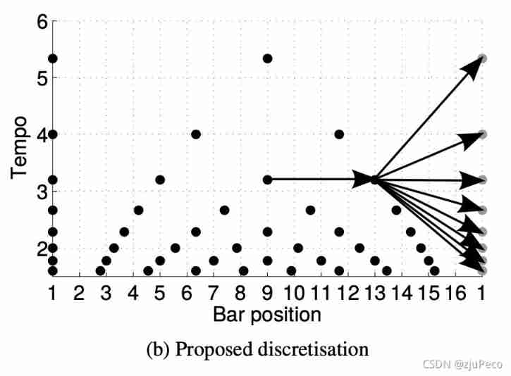
(1) Improvement of position resolution
To put it bluntly, it is to adjust one according to the speed bar To be divided into several parts . From the picture 4-2 You can see from the horizontal of ,tempo The bigger ,bar position The more sparsely they are divided , On the contrary, the more dense . The division method is from the specific madmom From the realization of , Don't read what the paper says , What is said in the paper is a little vague .
""" max_bpm: User input , Represents the largest beats per minute, The default is 215 min_bpm: User input , The smallest beats per minute, The default is 55 fps: User input ,frame per second min_interval: To calculate the , The smallest frame per beat max_interval: To calculate the , maximal frame per beat """
# convert timing information to construct a beat state space
min_interval = 60. * fps / max_bpm # second per beat * frame per second = frame per beat
max_interval = 60. * fps / min_bpm
In the code slice above min_interval and max_interval By the largest bpm And the smallest bpm Identify each beat How many are divided into frames. One bar How many beats It is also input by the user , So a bar Of bar positions It is determined according to different speeds .
(2) Improvement of speed resolution
Speed at min_bpm and max_bpm Within the scope of , Press log linear Is divided into . See this paragraph for specific implementation https://github.com/CPJKU/madmom/blob/master/madmom/features/beats_hmm.py#L66. It should be said that it is being implemented , There is no such thing as speed , All changed into positions . Different bpm There are different location points under ,log linear The object of is location .
(3) Speed stability
In order to ensure the stability of speed , The speed can only be in each beat The position of , Change depends on a distribution , This distribution is obtained from several experiments .
When Φ k ∈ B \Phi_k \in B Φk∈B when
P ( Φ ˙ k ∣ Φ ˙ k − 1 ) = f ( Φ ˙ k , Φ ˙ k − 1 ) (4-6) P(\dot{\Phi}_k | \dot{\Phi}_{k-1}) = f(\dot{\Phi}_k, \dot{\Phi}_{k-1}) \tag{4-6} P(Φ˙k∣Φ˙k−1)=f(Φ˙k,Φ˙k−1)(4-6)
among f ( Φ ˙ k , Φ ˙ k − 1 ) f(\dot{\Phi}_k, \dot{\Phi}_{k-1}) f(Φ˙k,Φ˙k−1) It can be a variety of functions , The better effect is
f ( Φ ˙ k , Φ ˙ k − 1 ) = e x p ( − λ × ∣ Φ ˙ k Φ ˙ k − 1 − 1 ∣ ) (4-7) f(\dot{\Phi}_k, \dot{\Phi}_{k-1}) = exp(-\lambda \times |\frac{\dot{\Phi}_k}{\dot{\Phi}_{k-1}} - 1|) \tag{4-7} f(Φ˙k,Φ˙k−1)=exp(−λ×∣Φ˙k−1Φ˙k−1∣)(4-7)
It's not hard to see. , When Φ ˙ k − 1 = Φ ˙ k \dot{\Phi}_{k-1} = \dot{\Phi}_k Φ˙k−1=Φ˙k When the probability is maximum . λ ∈ [ 1 , 300 ] \lambda \in [1, 300] λ∈[1,300] It's a super parameter , Different λ \lambda λ Next f ( Φ ˙ k , Φ ˙ k − 1 ) f(\dot{\Phi}_k, \dot{\Phi}_{k-1}) f(Φ˙k,Φ˙k−1) The results are as follows 4-3 Shown .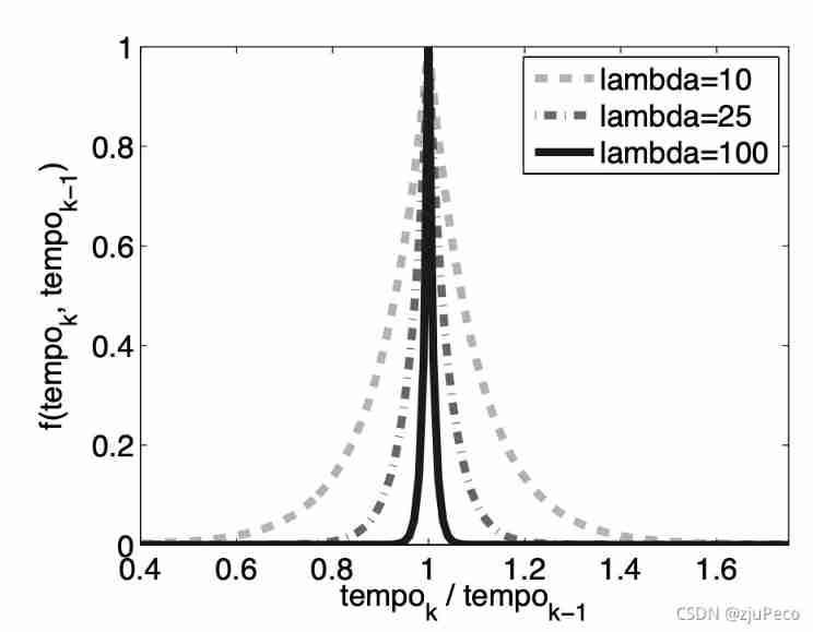
When Φ k ∉ B \Phi_k \notin B Φk∈/B when
P ( Φ ˙ k ∣ Φ ˙ k − 1 ) = { 1 , Φ ˙ k = Φ ˙ k − 1 0 , o t h e r w i s e (4-8) P(\dot{\Phi}_k | \dot{\Phi}_{k-1}) = \begin{cases} 1, & \dot{\Phi}_k = \dot{\Phi}_{k-1} \\ 0, & otherwise \end{cases} \tag{4-8} P(Φ˙k∣Φ˙k−1)={ 1,0,Φ˙k=Φ˙k−1otherwise(4-8)
It means that the speed does not change .
5 forecast
madmom The whole model is clearly divided into two parts ,DBNDownBeatTrackingProcessor and RNNDownBeatProcessor.RNNDownBeatProcessor It's ours RNN The Internet ,DBNDownBeatTrackingProcessor yes HMM Part of . On the macro level ,beats and downbeats The position of is by RNN Roughly determine , Then from HMM Determining the final position according to the condition of periodicity .RNN It can be understood as a partial understanding ,HMM It is a decision for the overall situation .
At the time of prediction , We will tell the model this song every bar Of beat There are several , If you're not sure , Just put beats_per_bar=[2,3,4,6] Fill in all , Let each model run to one side , Then take the one with the greatest probability .
At every beats_per_bar Next , We calculate an optimal hidden variable path
x 1 : K ∗ = a r g max x 1 : K ( x 1 : K ∣ y 1 : K ) (5-1) \bold{x}_{1:K}^* = arg\max_{x_{1:K}}(\bold{x}_{1:K} | \bold{y}_{1:K}) \tag{5-1} x1:K∗=argx1:Kmax(x1:K∣y1:K)(5-1)
Solve this with viterbi Algorithm will do .
The end result is
B ∗ = { k : x k ∗ ∈ B } (5-2) B^* = \{k : \bold{x}_k^* \in B\} \tag{5-2} B∗={ k:xk∗∈B}(5-2)
D ∗ = { k : x k ∗ ∈ D } (5-2) D^* = \{k : \bold{x}_k^* \in D\} \tag{5-2} D∗={ k:xk∗∈D}(5-2)
To determine the B ∗ B^* B∗ and D ∗ D^* D∗ after , And according to RNN Result , Correct the point to the nearby probability peak point .
When validating the model , Keep the error within 70ms All points within are considered correct .madmom The effect is still very good .
Reference material
[1] madmom implementation
[2] Joint Beat and Downbeat Tracking with Recurrent Neural Networks
[3] An Efficient State-Space Model for Joint Tempo and Meter Tracking
[4] Baidu Encyclopedia - Beats
[5] Bayesian Modelling of Temporal Structure in Musical Audio
[6] A Multi-model Approach to Beat Tracking Considering Heterogeneous Music Styles
边栏推荐
- ROS learning-6 detailed explanation of publisher programming syntax
- js获取元素
- Huawei equipment configures private IP routing FRR
- How to do Internet for small enterprises
- 柏瑞凱電子沖刺科創板:擬募資3.6億 汪斌華夫婦為大股東
- Day 1 of the 10 day smart lock project (understand the SCM stm32f401ret6 and C language foundation)
- 【Unity】打包WebGL项目遇到的问题及解决记录
- 华为设备配置IP和虚拟专用网混合FRR
- Learning notes 51 single chip microcomputer keyboard (non coding keyboard and coding keyboard, scanning mode of non coding keyboard, independent keyboard, matrix keyboard)
- CCF 201409-1: adjacent number pairs (100 points + problem solving ideas)
猜你喜欢

Review the history of various versions of ITIL, and find the key points for the development of enterprise operation and maintenance
![[pytorch]fixmatch code explanation - data loading](/img/0f/1165dbe4c7410a72d74123ec52dc28.jpg)
[pytorch]fixmatch code explanation - data loading

如何解决通过new Date()获取时间写出数据库与当前时间相差8小时问题【亲测有效】

Chapter7-11_ Deep Learning for Question Answering (2/2)

Viewing the ambition of Xiaodu technology from intelligent giant screen TV v86

柏瑞凯电子冲刺科创板:拟募资3.6亿 汪斌华夫妇为大股东

4.11 introduction to firmware image package

Sensor: sht30 temperature and humidity sensor testing ambient temperature and humidity experiment (code attached at the bottom)
![[the third day of actual combat of smart lock project based on stm32f401ret6 in 10 days] communication foundation and understanding serial port](/img/82/ed215078da0325b3adf95dcd6ffe30.jpg)
[the third day of actual combat of smart lock project based on stm32f401ret6 in 10 days] communication foundation and understanding serial port

10 days based on stm32f401ret6 smart lock project practice day 1 (environment construction and new construction)
随机推荐
[learning notes] xr872 GUI littlevgl 8.0 migration (file system)
Think: when do I need to disable mmu/i-cache/d-cache?
Day 1 of the 10 day smart lock project (understand the SCM stm32f401ret6 and C language foundation)
Bluetooth module: use problem collection
Understanding and thinking about multi-core consistency
Huawei equipment configures private IP routing FRR
cmake_ example
[pytorch] kaggle image classification competition arcface + bounding box code learning
华为设备配置私网IP路由FRR
[single chip microcomputer] single timer in front and back platform program framework to realize multi delay tasks
Viewing the ambition of Xiaodu technology from intelligent giant screen TV v86
Leetcode 93 recovery IP address
[the 4th day of the 10 day smart lock project based on stm32f401ret6] what is interrupt, interrupt service function, system tick timer
Basic exercises of test questions letter graphics ※
Interruption of 51 single chip microcomputer learning notes (external interruption, timer interruption, interrupt nesting)
C language compressed string is saved to binary file, and the compressed string is read from binary file and decompressed.
[printf function and scanf function] (learning note 5 -- standard i/o function)
Mac下搭建MySQL环境
The execution results of i+=2 and i++ i++ under synchronized are different
Mac使用Docker安装Oracle