当前位置:网站首页>Image recognition and detection -- Notes
Image recognition and detection -- Notes
2022-07-03 07:27:00 【Deer holding grass】
Image recognition and detection
1.Variable
stay Torch Medium Variable It is a place to store values that will change ( Basket ). The value inside will keep changing . The value of the inside , Namely Tensor tensor ( egg ).
import torch
from torch.autograd import Variable # torch  in  Variable  modular
#  Prepare eggs
tensor = torch.FloatTensor([[1,2],[3,4]])
#  Put the eggs in the basket , requires_grad Whether to participate in error back propagation ,  Do you want to calculate the gradient
variable = Variable(tensor, requires_grad=True)

print("Tensor:\n" + str(tensor))
print("\n")
print("Variable:\n" + str(variable))

2. Variable Calculation , gradient
t_out = torch.mean(tensor*tensor)       # x^2
v_out = torch.mean(variable*variable)   # x^2
print(t_out)
print(v_out)
up to now , We can't see any difference , But always remember , Variable When calculating , It silently builds a huge system step by step behind the background curtain , It's called a calculation chart , computational graph. What is this picture for ? It turns out that all the calculation steps ( node ) All connected , Finally, when the error is transmitted back , All at once variable The modification range ( gradient ) All worked out , and tensor There is no such ability .
v_out = torch.mean(variable*variable)#  It is a calculation step added to the calculation diagram ,  He contributed to the calculation of the reverse transmission of errors ,  Let's take an example :
v_out.backward()    #  simulation  v_out  The error is transmitted in reverse

# v_out = torch.mean(variable*variable)  This is the definition
# v_out = 1/4 * sum(variable*variable)  This is the  v_out The actual mathematical formula of
#  Aim at  v_out  The gradient is :
# d(v_out)/d(variable) = 1/4*2*variable = variable/2
print("variable.grad:\n")
print(variable.grad)    #  initial  Variable  Gradient of
3. obtain Variable The data in it
direct print(variable) Only output Variable Data in form , In many cases, it is useless ( For example, I want to use plt drawing ), So we need to switch , Turn it into tensor form
print(variable)     # Variable  form
print(variable.data)    # tensor  form
print(variable.data.numpy())    # numpy  form
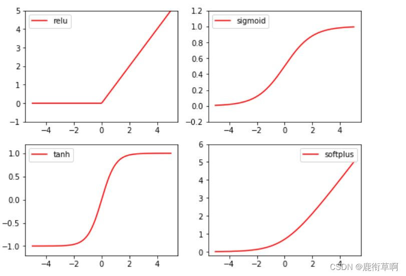
4. Excitation function (Activation)
Common excitation functions :Relu, Sigmoid, Tanh, Softplus
import torch
import torch.nn.functional as F     #  The excitation functions are all here
from torch.autograd import Variable

x = torch.linspace(-5, 5, 200)  # x data (tensor), shape=(100, 1)
x = Variable(x)
print(x.shape)

import matplotlib.pyplot as plt

plt.figure(1, figsize=(8, 6))
plt.subplot(221)
plt.plot(x_np, y_relu, c='red', label='relu')
plt.ylim((-1, 5))
plt.legend(loc='best')

plt.subplot(222)
plt.plot(x_np, y_sigmoid, c='red', label='sigmoid')
plt.ylim((-0.2, 1.2))
plt.legend(loc='best')

plt.subplot(223)
plt.plot(x_np, y_tanh, c='red', label='tanh')
plt.ylim((-1.2, 1.2))
plt.legend(loc='best')

plt.subplot(224)
plt.plot(x_np, y_softplus, c='red', label='softplus')
plt.ylim((-0.2, 6))
plt.legend(loc='best')

plt.show()
5. Regression
import torch
import torch.nn.functional as F     #  The excitation functions are all here
import matplotlib.pyplot as plt
x = torch.unsqueeze(torch.linspace(-1, 1, 100), dim=1)  # x data (tensor), shape=(100, 1)
y = x.pow(2) + 0.2*torch.rand(x.size())                 # noisy y data (tensor), shape=(100, 1)

#  drawing
plt.scatter(x.data.numpy(), y.data.numpy())
plt.show()

torch.unsqueeze(input, dim, out=None) effect : Expand dimensions Returns a new tensor , Insert a dimension into the given location of the input 1 Be careful : Return tensor and input tensor share memory , So changing the content of one will change the other
torch.linspace(start, end, steps=100, out=None) Return to one 1 D tensor , Included in interval start and end Evenly spaced on step A little bit . The length of the output tensor is determined by steps decision .
Parameters : start (float) - The starting point of the interval end (float) - The end of the interval steps (int) - stay start and end Number of samples generated between out (Tensor, optional) - The result tensor
torch.rand(*sizes, out=None) → Tensor Return a tensor , Contains the from interval [0,1) A set of random numbers extracted from the uniform distribution of , The shape consists of variable parameters sizes Definition .
Parameters : sizes (int…) – Sequence of integers , Defines the output shape out (Tensor, optinal) - The result tensor
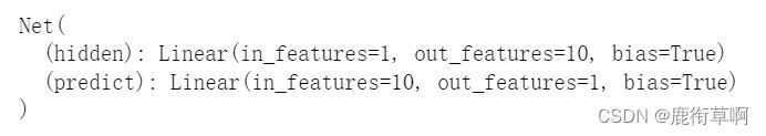
6. Building neural networks
class Net(torch.nn.Module):  #  Inherit  torch  Of  Module
    def __init__(self, n_feature, n_hidden, n_output):
        super(Net, self).__init__()     #  Inherit  __init__  function
        #  Define the form of each layer
        self.hidden = torch.nn.Linear(n_feature, n_hidden)   #  Hidden layer linear output
        self.predict = torch.nn.Linear(n_hidden, n_output)   #  Output layer linear output

    def forward(self, x):   #  It's also  Module  Medium  forward  function
        #  Forward propagation input value ,  The neural network analyzes the output value
        x = F.relu(self.hidden(x))      #  Excitation function ( The linear value of the hidden layer )
        x = self.predict(x)             #  Output value
        return x

net = Net(n_feature=1, n_hidden=10, n_output=1)

print(net)
net2 = torch.nn.Sequential(
    torch.nn.Linear(1, 10),
    torch.nn.ReLU(),
    torch.nn.Linear(10, 1)
)
print(net2)

7. Training network
# optimizer  It's a training tool
optimizer = torch.optim.SGD(net.parameters(), lr=0.2)  #  Pass in  net  All parameters of ,  Learning rate
loss_func = torch.nn.MSELoss()      #  Calculation formula of error between predicted value and real value  ( Mean square error )

epochs = 200

plt.ion()   #  drawing
plt.show()

for t in range(epochs):
    prediction = net(x)     #  Feeding  net  Training data  x,  Output predicted value

    loss = loss_func(prediction, y)     #  Calculate the error between the two

    optimizer.zero_grad()   #  Clear the residual update parameter value of the previous step
    loss.backward()         #  Error back propagation ,  Calculate parameter update values
    optimizer.step()        #  Apply the parameter update value to  net  Of  parameters  On

    # drawing
    if t % 5 == 0:
        # plot and show learning process
        plt.cla()
        plt.scatter(x.data.numpy(), y.data.numpy())
        plt.plot(x.data.numpy(), prediction.data.numpy(), 'r-', lw=5)
        plt.text(0.5, 0, 'Loss=%.4f' % loss.data.numpy(), fontdict={
    'size': 20, 'color':  'red'})
        plt.pause(0.1)
边栏推荐
- Dora (discover offer request recognition) process of obtaining IP address
- 最全SQL与NoSQL优缺点对比
- Use of file class
- TypeScript let与var的区别
- Lombok cooperates with @slf4j and logback to realize logging
- 7.2 brush two questions
- Advanced APL (realize group chat room)
- Distributed lock
- LeetCode
- TCP cumulative acknowledgement and window value update
猜你喜欢

Qtip2 solves the problem of too many texts

C code production YUV420 planar format file

SecureCRT取消Session记录的密码
【开发笔记】基于机智云4G转接板GC211的设备上云APP控制

为什么说数据服务化是下一代数据中台的方向?
![[solved] unknown error 1146](/img/f1/b8dd3ca8359ac9eb19e1911bd3790a.png)
[solved] unknown error 1146

《指环王:力量之戒》新剧照 力量之戒铸造者亮相

Comparison of advantages and disadvantages between most complete SQL and NoSQL
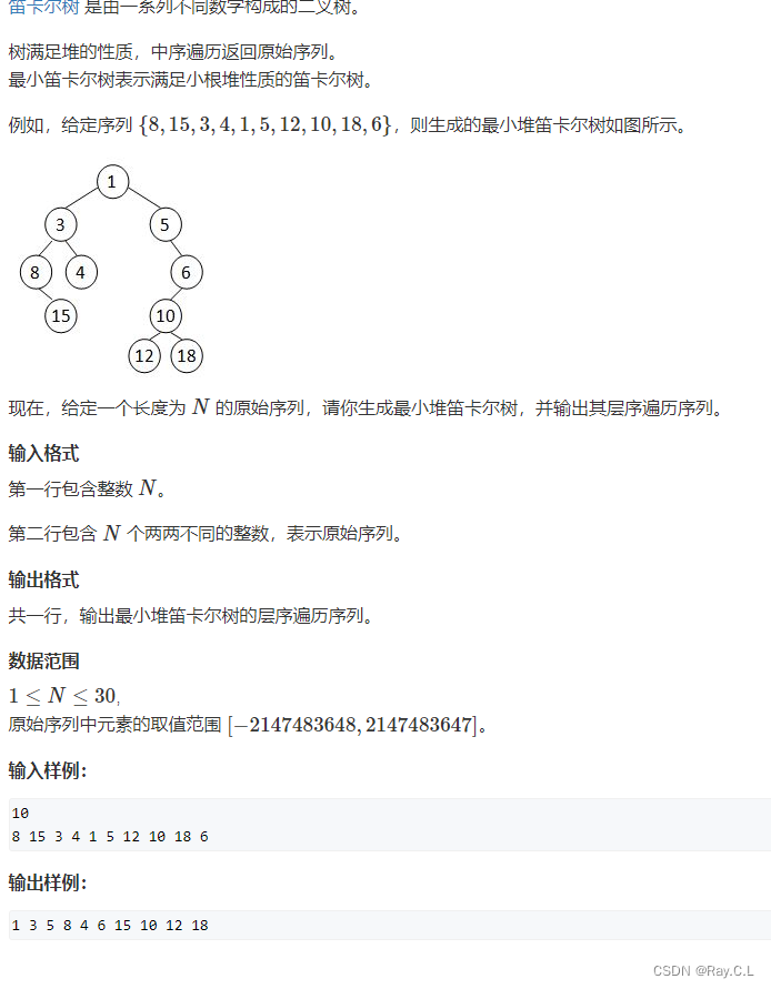
4279. 笛卡尔树

Store WordPress media content on 4everland to complete decentralized storage
随机推荐
2. E-commerce tool cefsharp autojs MySQL Alibaba cloud react C RPA automated script, open source log
【开发笔记】基于机智云4G转接板GC211的设备上云APP控制
Various postures of CS without online line
Some experiences of Arduino soft serial port communication
Raspberry pie update tool chain
Pat grade a real problem 1166
Comparison of advantages and disadvantages between most complete SQL and NoSQL
Common methods of file class
Advanced APL (realize group chat room)
Read config configuration file of vertx
JUnit unit test of vertx
La différence entre le let Typescript et le Var
Distributed lock
VMware virtual machine installation
专题 | 同步 异步
[set theory] Stirling subset number (Stirling subset number concept | ball model | Stirling subset number recurrence formula | binary relationship refinement relationship of division)
Use of file class
Vertx's responsive redis client
[solved] win10 cannot find a solution to the local group policy editor
Introduction of buffer flow