使用贝叶斯优化进行深度神经网络超参数优化

在本文中，我们将深入研究超参数优化。

为了方便起见本文将使用 Tensorflow 中包含的 Fashion MNIST[1] 数据集。该数据集在训练集中包含 60,000 张灰度图像，在测试集中包含 10,000 张图像。每张图片代表属于 10 个类别之一的单品（“T 恤/上衣”、“裤子”、“套头衫”等）。因此这是一个多类分类问题。

这里简单介绍准备数据集的步骤，因为本文的主要内容是超参数的优化，所以这部分只是简单介绍流程，一般情况下，流程如下：

• 加载数据。
• 分为训练集、验证集和测试集。
• 将像素值从 0–255 标准化到 0–1 范围。
• One-hot 编码目标变量。

#load data
(train_images, train_labels), (test_images, test_labels) = fashion_mnist.load_data()

# split into train, validation and test sets
train_x, val_x, train_y, val_y = train_test_split(train_images, train_labels, stratify=train_labels, random_state=48, test_size=0.05)
(test_x, test_y)=(test_images, test_labels)

# normalize pixels to range 0-1
train_x = train_x / 255.0
val_x = val_x / 255.0
test_x = test_x / 255.0

#one-hot encode target variable
train_y = to_categorical(train_y)
val_y = to_categorical(val_y)
test_y = to_categorical(test_y)

我们所有训练、验证和测试集的形状是：

print(train_x.shape)  #(57000, 28, 28)
print(train_y.shape)  #(57000, 10)
print(val_x.shape)    #(3000, 28, 28)
print(val_y.shape)    #(3000, 10)
print(test_x.shape)   #(10000, 28, 28)
print(test_y.shape)   #(10000, 10)

现在，我们将使用 Keras Tuner 库 [2]：它将帮助我们轻松调整神经网络的超参数：

pip install keras-tuner

Keras Tuner 需要 Python 3.6+ 和 TensorFlow 2.0+

超参数调整是机器学习项目的基础部分。有两种类型的超参数：

• 结构超参数：定义模型的整体架构（例如隐藏单元的数量、层数）
• 优化器超参数：影响训练速度和质量的参数（例如学习率和优化器类型、批量大小、轮次数等）

为什么需要超参数调优库？我们不能尝试所有可能的组合，看看验证集上什么是最好的吗？

这肯定是不行的因为深度神经网络需要大量时间来训练，甚至几天。如果在云服务器上训练大型模型，那么每个实验实验都需要花很多的钱。

因此，需要一种限制超参数搜索空间的剪枝策略。

keras-tuner提供了贝叶斯优化器。它搜索每个可能的组合，而是随机选择前几个。然后根据这些超参数的性能，选择下一个可能的最佳值。因此每个超参数的选择都取决于之前的尝试。根据历史记录选择下一组超参数并评估性能，直到找到最佳组合或到达最大试验次数。我们可以使用参数“max_trials”来配置它。

除了贝叶斯优化器之外，keras-tuner还提供了另外两个常见的方法：RandomSearch 和 Hyperband。我们将在本文末尾讨论它们。

接下来就是对我们的网络应用超参数调整。我们尝试两种网络架构，标准多层感知器（MLP）和卷积神经网络（CNN）。

首先让我们看看基线 MLP 模型是什么：

model_mlp = Sequential()
model_mlp.add(Flatten(input_shape=(28, 28)))
model_mlp.add(Dense(350, activation='relu'))
model_mlp.add(Dense(10, activation='softmax'))
print(model_mlp.summary())
model_mlp.compile(optimizer="adam",loss='categorical_crossentropy')

调优过程需要两种主要方法：

hp.Int()：设置超参数的范围，其值为整数 - 例如，密集层中隐藏单元的数量：

model.add(Dense(units = hp.Int('dense-bot', min_value=50, max_value=350, step=50))

hp.Choice()：为超参数提供一组值——例如，Adam 或 SGD 作为最佳优化器？

hp_optimizer=hp.Choice('Optimizer', values=['Adam', 'SGD'])

在我们的 MLP 示例中，我们测试了以下超参数：

• 隐藏层数：1-3
• 第一密集层大小：50–350
• 第二和第三密集层大小：50–350
• Dropout：0、0.1、0.2
• 优化器：SGD(nesterov=True,momentum=0.9) 或 Adam
• 学习率：0.1、0.01、0.001

代码如下：

model = Sequential()

model.add(Dense(units = hp.Int('dense-bot', min_value=50, max_value=350, step=50), input_shape=(784,), activation='relu'))

for i in range(hp.Int('num_dense_layers', 1, 2)):
  model.add(Dense(units=hp.Int('dense_' + str(i), min_value=50, max_value=100, step=25), activation='relu'))
  model.add(Dropout(hp.Choice('dropout_'+ str(i), values=[0.0, 0.1, 0.2])))

model.add(Dense(10,activation="softmax"))

hp_optimizer=hp.Choice('Optimizer', values=['Adam', 'SGD'])

if hp_optimizer == 'Adam':
    hp_learning_rate = hp.Choice('learning_rate', values=[1e-1, 1e-2, 1e-3])
elif hp_optimizer == 'SGD':
    hp_learning_rate = hp.Choice('learning_rate', values=[1e-1, 1e-2, 1e-3])
    nesterov=True
    momentum=0.9

这里需要注意第 5 行的 for 循环：让模型决定网络的深度！

最后，就是运行了。请注意我们之前提到的 max_trials 参数。

model.compile(optimizer = hp_optimizer, loss='categorical_crossentropy', metrics=['accuracy'])

tuner_mlp = kt.tuners.BayesianOptimization(
    model,
    seed=random_seed,
    objective='val_loss',
    max_trials=30,
    directory='.',
    project_name='tuning-mlp')
tuner_mlp.search(train_x, train_y, epochs=50, batch_size=32, validation_data=(dev_x, dev_y), callbacks=callback)

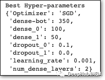
我们得到结果

这个过程用尽了迭代次数，大约需要 1 小时才能完成。我们还可以使用以下命令打印模型的最佳超参数：

best_mlp_hyperparameters = tuner_mlp.get_best_hyperparameters(1)[0]
print("Best Hyper-parameters")
best_mlp_hyperparameters.values

现在我们可以使用最优超参数重新训练我们的模型：

model_mlp = Sequential()

model_mlp.add(Dense(best_mlp_hyperparameters['dense-bot'], input_shape=(784,), activation='relu'))

for i in range(best_mlp_hyperparameters['num_dense_layers']):
  model_mlp.add(Dense(units=best_mlp_hyperparameters['dense_' +str(i)], activation='relu'))
  model_mlp.add(Dropout(rate=best_mlp_hyperparameters['dropout_' +str(i)]))
  
model_mlp.add(Dense(10,activation="softmax"))

model_mlp.compile(optimizer=best_mlp_hyperparameters['Optimizer'], loss='categorical_crossentropy',metrics=['accuracy'])
history_mlp= model_mlp.fit(train_x, train_y, epochs=100, batch_size=32, validation_data=(dev_x, dev_y), callbacks=callback)

或者，我们可以用这些参数重新训练我们的模型：

model_mlp=tuner_mlp.hypermodel.build(best_mlp_hyperparameters)

history_mlp=model_mlp.fit(train_x, train_y, epochs=100, batch_size=32, 
                           validation_data=(dev_x, dev_y), callbacks=callback)

然后测试准确率

mlp_test_loss, mlp_test_acc = model_mlp.evaluate(test_x,  test_y, verbose=2)
print('\nTest accuracy:', mlp_test_acc)

# Test accuracy: 0.8823

与基线的模型测试精度相比：

基线 MLP 模型：86.6 %最佳 MLP 模型：88.2 %。测试准确度的差异约为 3%！

下面我们使用相同的流程，将MLP改为CNN，这样可以测试更多参数。

首先，这是我们的基线模型：

model_cnn = Sequential()
model_cnn.add(Conv2D(32, (3, 3), activation='relu', input_shape=(28, 28, 1)))
model_cnn.add(MaxPooling2D((2, 2)))
model_cnn.add(Flatten())
model_cnn.add(Dense(100, activation='relu'))
model_cnn.add(Dense(10, activation='softmax'))
model_cnn.compile(optimizer="adam", loss='categorical_crossentropy', metrics=['accuracy'])

基线模型 包含卷积和池化层。对于调优，我们将测试以下内容：

1. 卷积、MaxPooling 和 Dropout 层的“块”数
2. 每个块中 Conv 层的过滤器大小：32、64
3. 转换层上的有效或相同填充
4. 最后一个额外层的隐藏层大小：25-150，乘以 25
5. 优化器：SGD（nesterov=True，动量=0.9）或 Adam
6. 学习率：0.01、0.001

model = Sequential()

model = Sequential()
model.add(Input(shape=(28, 28, 1)))

for i in range(hp.Int('num_blocks', 1, 2)):
    hp_padding=hp.Choice('padding_'+ str(i), values=['valid', 'same'])
    hp_filters=hp.Choice('filters_'+ str(i), values=[32, 64])

    model.add(Conv2D(hp_filters, (3, 3), padding=hp_padding, activation='relu', kernel_initializer='he_uniform', input_shape=(28, 28, 1)))
    model.add(MaxPooling2D((2, 2)))
    model.add(Dropout(hp.Choice('dropout_'+ str(i), values=[0.0, 0.1, 0.2])))

model.add(Flatten())

hp_units = hp.Int('units', min_value=25, max_value=150, step=25)
model.add(Dense(hp_units, activation='relu', kernel_initializer='he_uniform'))

model.add(Dense(10,activation="softmax"))

hp_learning_rate = hp.Choice('learning_rate', values=[1e-2, 1e-3])
hp_optimizer=hp.Choice('Optimizer', values=['Adam', 'SGD'])

if hp_optimizer == 'Adam':
    hp_learning_rate = hp.Choice('learning_rate', values=[1e-2, 1e-3])
elif hp_optimizer == 'SGD':
    hp_learning_rate = hp.Choice('learning_rate', values=[1e-2, 1e-3])
    nesterov=True
    momentum=0.9

像以前一样，我们让网络决定它的深度。最大迭代次数设置为 100：

model.compile( optimizer=hp_optimizer,loss='categorical_crossentropy', metrics=['accuracy'])

tuner_cnn = kt.tuners.BayesianOptimization(
    model,
    objective='val_loss',
    max_trials=100,
    directory='.',
    project_name='tuning-cnn')

结果如下：

得到的超参数

最后使用最佳超参数训练我们的 CNN 模型：

model_cnn = Sequential()

model_cnn.add(Input(shape=(28, 28, 1)))

for i in range(best_cnn_hyperparameters['num_blocks']):
  hp_padding=best_cnn_hyperparameters['padding_'+ str(i)]
  hp_filters=best_cnn_hyperparameters['filters_'+ str(i)]

  model_cnn.add(Conv2D(hp_filters, (3, 3), padding=hp_padding, activation='relu', kernel_initializer='he_uniform', input_shape=(28, 28, 1)))
  model_cnn.add(MaxPooling2D((2, 2)))
  model_cnn.add(Dropout(best_cnn_hyperparameters['dropout_'+ str(i)]))

model_cnn.add(Flatten())
model_cnn.add(Dense(best_cnn_hyperparameters['units'], activation='relu', kernel_initializer='he_uniform'))

model_cnn.add(Dense(10,activation="softmax"))

model_cnn.compile(optimizer=best_cnn_hyperparameters['Optimizer'], 
                                                 loss='categorical_crossentropy', 
                                                 metrics=['accuracy'])
print(model_cnn.summary())

history_cnn= model_cnn.fit(train_x, train_y, epochs=50, batch_size=32, validation_data=(dev_x, dev_y), callbacks=callback)

检查测试集的准确率：

cnn_test_loss, cnn_test_acc = model_cnn.evaluate(test_x,  test_y, verbose=2)
print('\nTest accuracy:', cnn_test_acc)

# Test accuracy: 0.92

与基线的 CNN 模型测试精度相比：

1. 基线 CNN 模型：90.8 %
2. 最佳 CNN 模型：92%

我们看到优化模型的性能提升！

除了准确性之外，我们还可以看到优化的效果很好，因为：

在每种情况下都选择了一个非零的 Dropout 值，即使我们也提供了零 Dropout。这是意料之中的，因为 Dropout 是一种减少过拟合的机制。有趣的是，最好的 CNN 架构是标准CNN，其中过滤器的数量在每一层中逐渐增加。这是意料之中的，因为随着后续层的增加，模式变得更加复杂（这也是我们在学习各种模型和论文时被证明的结果）需要更多的过滤器才能捕获这些模式组合。

以上例子也说明Keras Tuner 是使用 Tensorflow 优化深度神经网络的很好用的工具。

我们上面也说了本文选择是贝叶斯优化器。但是还有两个其他的选项：

RandomSearch：随机选择其中的一些来避免探索超参数的整个搜索空间。但是，它不能保证会找到最佳超参数

Hyperband：选择一些超参数的随机组合，并仅使用它们来训练模型几个 epoch。然后使用这些超参数来训练模型，直到用尽所有 epoch 并从中选择最好的。

最后数据集地址和keras_tuner的文档如下

https://avoid.overfit.cn/post/c3f904fab4f84914b8a1935f8670582f

作者：Nikos Kafritsas