当前位置:网站首页>[0 basic operations research] [super detail] column generation
[0 basic operations research] [super detail] column generation
2022-07-27 15:33:00 【ymzhu385】
Catalog
Column generation (Column generation) It is an effective algorithm for solving large linear programs .
Related courses
Related literature
- Column generation(wikipedia)
- dried food | 10 Minutes will give you a thorough understanding of column generation( Column generation ) The principle of the algorithm java Code
- Column generation and branch pricing
- Linear programming skills : Column generation (Column Generation)
- Principle of column generation algorithm ( Simplex basis )
- Column generation (Column Generation) Algorithm
- 【Column Generation reflection -02】| Understand... From the perspective of duality Cutting Stock Problem【 An updated version 】
- Gilmore P C, Gomory R E. A linear programming approach to the cutting-stock problem[J]. Operations research, 1961, 9(6): 849-859.
- Operations research says The first 21 period | Algorithm introduction column generation algorithm
Preface
I've always wanted to share with you Column generation (Column generation), I also searched many documents all over the Internet 、 video 、 Papers, etc . Most tutorials are highly abstract , It requires a lot of basic knowledge to understand , So write an article as much as possible 0 Basic sharing , I hope I can help you who are also engaged in related industries .
Someone must ask , Is there any Row generation algorithm ? Of course. !!! I'll share it with you when I have a chance !!!——@ Pig Rush
Start with an example :Cutting Stock Problem
Problem description
The seller has 3 A length of wood :9cm(5 element ),14cm(9 element ),16cm(10 element ).
Buyers need wood :4cm(30 root ),5cm(20 root ),7cm(40 root ).
So the seller needs to pass Cut wood Meet the needs of buyers , And the seller hopes Lowest cost So as to benefit the most .
analysis
First, let's think briefly , A piece of 9cm How many kinds of wood cutting methods can meet the needs of buyers 4cm,5cm,7cm
| cost( element ) | Length of wood before cutting (cm) | 4cm Quantity of wood | 5cm Quantity of wood | 7cm Quantity of wood |
|---|---|---|---|---|
| 5 | 9 | 1 | 0 | 0 |
| 5 | 9 | 2 | 0 | 0 |
| 5 | 9 | 0 | 1 | 0 |
| 5 | 9 | 1 | 1 | 0 |
| 5 | 9 | 0 | 0 | 1 |
In line with the traditional Chinese virtue of not wasting , obviously The cut of the second line is better than the first line Some (^U^)ノ~YO
We usually call a cutting method cutting pattern.
All right. , Then it was very easy After that ( Only keep the better pattern).
All Cutting Pattern:
| cost( element ) | Length of wood before cutting (cm) | 4cm Quantity of wood | 5cm Quantity of wood | 7cm Quantity of wood | Symbol |
|---|---|---|---|---|---|
| 5 | 9 | 2 | 0 | 0 | x 1 x_1 x1 |
| 5 | 9 | 1 | 1 | 0 | x 2 x_2 x2 |
| 5 | 9 | 0 | 0 | 1 | x 3 x_3 x3 |
| 9 | 14 | 3 | 0 | 0 | x 4 x_4 x4 |
| 9 | 14 | 2 | 1 | 0 | x 5 x_5 x5 |
| 9 | 14 | 1 | 2 | 0 | x 6 x_6 x6 |
| 9 | 14 | 1 | 0 | 1 | x 7 x_7 x7 |
| 9 | 14 | 0 | 1 | 1 | x 8 x_8 x8 |
| 9 | 14 | 0 | 0 | 2 | x 9 x_9 x9 |
| 10 | 16 | 4 | 0 | 0 | x 10 x_{10} x10 |
| 10 | 16 | 2 | 0 | 1 | x 11 x_{11} x11 |
| 10 | 16 | 1 | 1 | 1 | x 12 x_{12} x12 |
| 10 | 16 | 0 | 3 | 0 | x 13 x_{13} x13 |
So we just need to start from All Cutting Pattern It's sure Every Pattern How many times does it take That's it .( for instance : such as x 1 = 30 \bm{x_1=30} x1=30 On behalf of us, we use the 1 Cut it in a different way 30 root 9cm Length of wood ).
Our goal is to use The least money Complete the buyer's needs , That is, every one of them Pattern Of c o s t × Number \bm{cost\times }\textbf{ Number } cost× Number The sum of .
5 x 1 + 5 x 2 + 5 x 3 + 9 x 4 + 9 x 5 + 9 x 6 + 9 x 7 + 9 x 8 + 9 x 9 + 10 x 10 + 10 x 11 + 10 x 12 + 10 x 13 5x_1+5x_2+5x_3+9x_4+9x_5+9x_6+9x_7+9x_8+9x_9+10x_{10}+10x_{11}+10x_{12}+10x_{13} 5x1+5x2+5x3+9x4+9x5+9x6+9x7+9x8+9x9+10x10+10x11+10x12+10x13
In addition, we need Meet the requirements of the number of buyers .
4cm More than 30 root :
2 x 1 + x 2 + 0 x 3 + 3 x 4 + 2 x 5 + x 6 + x 7 + 0 x 8 + 0 x 9 + 4 x 10 + 2 x 11 + x 12 + 0 x 13 ≥ 30 2x_1+x_2+0x_3+3x_4+2x_5+x_6+x_7+0x_8+0x_9+4x_{10}+2x_{11}+x_{12}+0x_{13}\geq 30 2x1+x2+0x3+3x4+2x5+x6+x7+0x8+0x9+4x10+2x11+x12+0x13≥30
5cm More than 20 root :
0 x 1 + x 2 + 0 x 3 + 0 x 4 + x 5 + 2 x 6 + 0 x 7 + x 8 + 0 x 9 + 0 x 10 + 0 x 11 + x 12 + 3 x 13 ≥ 20 0x_1+x_2+0x_3+0x_4+x_5+2x_6+0x_7+x_8+0x_9+0x_{10}+0x_{11}+x_{12}+3x_{13}\geq 20 0x1+x2+0x3+0x4+x5+2x6+0x7+x8+0x9+0x10+0x11+x12+3x13≥20
7cm More than 70 root :
0 x 1 + 0 x 2 + x 3 + 0 x 4 + 0 x 5 + 0 x 6 + x 7 + x 8 + 2 x 9 + 0 x 10 + x 11 + x 12 + 0 x 13 ≥ 40 0x_1+0x_2+x_3+0x_4+0x_5+0x_6+x_7+x_8+2x_9+0x_{10}+x_{11}+x_{12}+0x_{13}\geq 40 0x1+0x2+x3+0x4+0x5+0x6+x7+x8+2x9+0x10+x11+x12+0x13≥40
modeling
Master Problem(MP)
Based on the above analysis , We already have decision variables x i x_i xi, We have the objective function The least money , We also have corresponding constraints Meet the requirements of the number of buyers , So we can model !!!
Defining decision variables x i \bm{x_i} xi In order to use the i i i Kind of Pattern Root number of .
min 5 x 1 + 5 x 2 + 5 x 3 + 9 x 4 + 9 x 5 + 9 x 6 + 9 x 7 + 9 x 8 + 9 x 9 + 10 x 10 + 10 x 11 + 10 x 12 + 10 x 13 \min{5x_1+5x_2+5x_3+9x_4+9x_5+9x_6+9x_7+9x_8+9x_9+10x_{10}+10x_{11}+10x_{12}+10x_{13}} min5x1+5x2+5x3+9x4+9x5+9x6+9x7+9x8+9x9+10x10+10x11+10x12+10x13
s . t . s.t. s.t.
2 x 1 + x 2 + 0 x 3 + 3 x 4 + 2 x 5 + x 6 + x 7 + 0 x 8 + 0 x 9 + 4 x 10 + 2 x 11 + x 12 + 0 x 13 ≥ 30 2x_1+x_2+0x_3+3x_4+2x_5+x_6+x_7+0x_8+0x_9+4x_{10}+2x_{11}+x_{12}+0x_{13}\geq 30 2x1+x2+0x3+3x4+2x5+x6+x7+0x8+0x9+4x10+2x11+x12+0x13≥30
0 x 1 + x 2 + 0 x 3 + 0 x 4 + x 5 + 2 x 6 + 0 x 7 + x 8 + 0 x 9 + 0 x 10 + 0 x 11 + x 12 + 3 x 13 ≥ 20 0x_1+x_2+0x_3+0x_4+x_5+2x_6+0x_7+x_8+0x_9+0x_{10}+0x_{11}+x_{12}+3x_{13}\geq 20 0x1+x2+0x3+0x4+x5+2x6+0x7+x8+0x9+0x10+0x11+x12+3x13≥20
0 x 1 + 0 x 2 + x 3 + 0 x 4 + 0 x 5 + 0 x 6 + x 7 + x 8 + 2 x 9 + 0 x 10 + x 11 + x 12 + 0 x 13 ≥ 40 0x_1+0x_2+x_3+0x_4+0x_5+0x_6+x_7+x_8+2x_9+0x_{10}+x_{11}+x_{12}+0x_{13}\geq 40 0x1+0x2+x3+0x4+0x5+0x6+x7+x8+2x9+0x10+x11+x12+0x13≥40
x i ∈ N x_i\in\mathbb{N} xi∈N
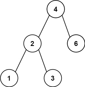
Each column :The number of times a feasible cutting scheme needs to be executed, perhapsHow many bars use this cutting scheme
Every line :The need for a bar must be met
Restricted Master Problem(RMP)
occasionally MP Will be very large , So we consider how to use several Pattern Get a feasible solution ( It may not be the optimal solution ), Then we have this feasible solution, and then we can see in turn if we add others Pattern Will there be a better solution , And directly solve MP The feasible solution may not be obtained in a given time .
So we follow this idea to build RMP( Pay attention to what we choose Pattern At least one feasible solution can be obtained ):
Defining decision variables x i \bm{x_i} xi In order to use the i i i Kind of Pattern Root number of .
min 5 x 1 + 5 x 2 + 5 x 3 \min{5x_1+5x_2+5x_3} min5x1+5x2+5x3
s . t . s.t. s.t.
2 x 1 + x 2 + 0 x 3 ≥ 30 2x_1+x_2+0x_3\geq 30 2x1+x2+0x3≥30
0 x 1 + x 2 + 0 x 3 ≥ 20 0x_1+x_2+0x_3\geq 20 0x1+x2+0x3≥20
0 x 1 + 0 x 2 + x 3 ≥ 40 0x_1+0x_2+x_3\geq 40 0x1+0x2+x3≥40
x i ∈ N x_i\in\mathbb{N} xi∈N
Restricted Linear Master Problem(RLMP)
The conventional column generation method is to solve LP The problem of , At this time, we do some proper relaxation ( That is to say x i ∈ N x_i\in\mathbb{N} xi∈N become x i ≥ 0 x_i\geq 0 xi≥0).
So we follow this idea to build RLMP( it is to be noted that RLMP The feasible solution of is not necessarily RMP Feasible solution of , But we just need to round up the solution ):
Defining decision variables x i \bm{x_i} xi In order to use the i i i Kind of Pattern Root number of .
min 5 x 1 + 5 x 2 + 5 x 3 \min{5x_1+5x_2+5x_3} min5x1+5x2+5x3
s . t . s.t. s.t.
2 x 1 + x 2 + 0 x 3 ≥ 30 2x_1+x_2+0x_3\geq 30 2x1+x2+0x3≥30
0 x 1 + x 2 + 0 x 3 ≥ 20 0x_1+x_2+0x_3\geq 20 0x1+x2+0x3≥20
0 x 1 + 0 x 2 + x 3 ≥ 40 0x_1+0x_2+x_3\geq 40 0x1+0x2+x3≥40
x i ≥ 0 x_i\geq 0 xi≥0
Then we can use LP solver Directly solve the above model ( Here I use Clp For example , Of course, you can use your favorite solver )
( In order to make the typesetting neat and convenient for reading , I will put the code at the end of the text )
Run directly to get 
In theory, we should treat the result
Round up, But we will get relaxedMPRounding after solution will be more convenient and efficient , So we don't do it hereRound up( But it seems that the solution is an integer Σ(⊙▽⊙"a——@ Pig Rush ):
O b j e c t i v e v a l u e = 325 Objective \: value = 325 Objectivevalue=325
x 1 = 5 x_1 = 5 x1=5
x 2 = 20 x_2 = 20 x2=20
x 3 = 40 x_3 = 40 x3=40
Let's try to explain solution The meaning of :use 5 individual Pattern 1( That is to say, I chose 5 root 9cm Of wood , Cut each into 2 individual 4cm), Similar again 20 individual Pattern 2 and 40 individual Pattern 3, Such a choice can minimize our total cost ——325 element .
Dual of Restricted Linear Master Problem
Now let's consider from another angle
RMP.
【 The seller 】 Buy the finished product directly ( Cut wood ), Sell it to customers , Similar middlemen .
【 The seller 】 The goal is : At most, how much money do you spend to buy finished products and earn more than you produce yourself .
【 The seller 】 constraint : We need to set a psychological price for the finished product . These psychological prices must meet :For any cutting scheme , Money to buy finished products <= Money produced by oneself.( for instance , Seller flower 5 Yuan to buy 1 root 9cm The wood can be cut into 2 individual 4cm finished product , That is to say, if the seller purchases directly 2 individual 4cm The price of finished products exceeds 5 Yuan, it's better to produce it yourself . Write a formula : 2 y 1 ≤ 5 2y_1\leq 5 2y1≤5, among y 1 \bm{y_1} y1 by 4cm Psychological price of wood )
————————————————————————————————————————————————————————
Defining decision variables y i \bm{y_i} yi Respectively 4cm(30 root ),5cm(20 root ),7cm(40 root ) Psychological price of wood .
max 30 y 1 + 20 y 2 + 40 y 3 \max{30y_1+20y_2+40y_3} max30y1+20y2+40y3
s . t . s.t. s.t.
2 y 1 + 0 y 2 + 0 y 3 ≤ 5 2y_1+0y_2+0y_3\leq 5 2y1+0y2+0y3≤5
y 1 + y 2 + 0 y 3 ≤ 5 y_1+y_2+0y_3\leq 5 y1+y2+0y3≤5
0 y 1 + 0 y 2 + y 3 ≤ 5 0y_1+0y_2+y_3\leq 5 0y1+0y2+y3≤5
y i ≥ 0 y_i\geq 0 yi≥0
Solve directly :
O b j e c t i v e v a l u e = 325 Objective \: value = 325 Objectivevalue=325
y 1 = 2.5 y_1 = 2.5 y1=2.5
y 2 = 2.5 y_2 = 2.5 y2=2.5
y 3 = 5.0 y_3 = 5.0 y3=5.0
Let's try to explain solution The meaning of :4cm、5cm、7cm The psychological prices of finished wood are 2.5 element 、2.5 element 、5 element , Most flowers 325 Yuan to buy finished products to earn more than their own production .That is, as long asPrice ratio 2.5 element 、2.5 element 、5 Yuan is low , The seller makes money.
Subproblem
- The meaning of simplex method test number : The product ( Variable ) The difference between the market price of and the implied cost of the product . The market price is higher than the implied cost , That is, when the inspection number is greater than zero , Then the product can be put into production .
- The test number of the original problem corresponds to a basic solution of its dual problem
If you know the concept of test number , Will soon understand subproblem, But here I'll assume you don't know , Try to make you understand in the simplest way ——@ Pig Rush
stay
dualIn the question, we calculate the psychological price of the finished product . Next, we want to know whether there is a more economical Pattern.
First, let's think about how to judge a Pattern Is it more economical .
Example 1:9cm The complete waste of wood is also a kind of Pattern, But one 9cm The wood should be 5 element , In other words, the seller lost 5 element .
Example 2:Pattern 9:14cm Wood (9 element ) Cut into 2 root 7cm finished product ( Use Pattern 1、2、3 Of 7cm Psychological price is 5 element ). That is, sellers only use Pattern 1、2、3 These three cutting methods , Just use less than 5 Yuan price purchase 7cm Selling it again is more profitable than cutting it yourself , And if you add Pattern 9, If the seller uses 5 The price of yuan is not as good as using it directly Pattern 9 To make money , It must be lower than 4.5 element (9 element /2) For the price of 7cm Selling it again is more profitable than cutting it yourself .
With the above two examples, we have gradually clarified how to judge a Pattern Is it more economical .
In other words, our goal is to find a new Pattern:new Pattern The finished product after cutting is old Pattern Psychological price under > new Pattern The price of
Defining decision variables a j \bm{a_{j}} aj It's new. Pattern After cutting 4cm,5cm,7cm The amount of wood .
new Pattern The finished product after cutting is old Pattern Psychological price under 【 2.5 a 1 + 2.5 a 2 + 5 a 3 2.5a_1+2.5a_2+5a_3 2.5a1+2.5a2+5a3】> new Pattern The price of 【9 element (14cm)】
namely :
2.5 a 1 + 2.5 a 2 + 5 a 3 > 9 2.5a_1+2.5a_2+5a_3>9 2.5a1+2.5a2+5a3>9
⇒ 9 − ( 2.5 a 1 + 2.5 a 2 + 5 a 3 ) < 0 \Rightarrow 9-(2.5a_1+2.5a_2+5a_3)<0 ⇒9−(2.5a1+2.5a2+5a3)<0( To the left of the inequality sign we generally call itInspection number, This is what we often sayThe test number determines whether the solution is the optimal solution)
Here we use a trick of converting constraints into objective functions : Make z = 9 − ( 2.5 a 1 + 2.5 a 2 + 5 a 3 ) z=9-(2.5a_1+2.5a_2+5a_3) z=9−(2.5a1+2.5a2+5a3), If min z \min z minz Than 0 Also big , That means it doesn't exist z > 0 z>0 z>0 Solution , That is, there is no more economical Pattern.
new Pattern The total length after cutting cannot exceed the length of the original wood : 4 a 1 + 5 a 2 + 7 a 3 ≤ 14 4a_1+5a_2+7a_3\leq 14 4a1+5a2+7a3≤14
All in all :
min 9 − ( 2.5 a 1 + 2.5 a 2 + 5 a 3 ) \min{9-(2.5a_1+2.5a_2+5a_3)} min9−(2.5a1+2.5a2+5a3)
4 a 1 + 5 a 2 + 7 a 3 ≤ 14 4a_1+5a_2+7a_3\leq 14 4a1+5a2+7a3≤14
So we set up 9cm、14cm、16cm Of Subproblem :
————————————————————————————————————————————————————————
Subproblem 1(9cm,5 element )
Defining decision variables a j \bm{a_{j}} aj yes Pattern After cutting 4cm,5cm,7cm The amount of wood .
min z = 5 − ( 2.5 a 1 + 2.5 a 2 + 5 a 3 ) \min{z=5-(2.5a_1+2.5a_2+5a_3)} minz=5−(2.5a1+2.5a2+5a3)
s . t . s.t. s.t.
4 a 1 + 5 a 2 + 7 a 3 ≤ 9 4a_1+5a_2+7a_3\leq 9 4a1+5a2+7a3≤9
a i ∈ N a_i\in\mathbb{N} ai∈N
To solve the need to : a = ( 2 , 0 , 0 ) T , z = 0 a=(2,0,0)^T, z=0 a=(2,0,0)T,z=0
————————————————————————————————————————————————————————
Subproblem 2(14cm,9 element )
Defining decision variables a j \bm{a_{j}} aj yes Pattern After cutting 4cm,5cm,7cm The amount of wood .
min z = 9 − ( 2.5 a 1 + 2.5 a 2 + 5 a 3 ) \min{z=9-(2.5a_1+2.5a_2+5a_3)} minz=9−(2.5a1+2.5a2+5a3)
s . t . s.t. s.t.
4 a 1 + 5 a 2 + 7 a 3 ≤ 14 4a_1+5a_2+7a_3\leq 14 4a1+5a2+7a3≤14
a i ∈ N a_i\in\mathbb{N} ai∈N
To solve the need to : a = ( 0 , 0 , 2 ) T , z = − 1 \bm{a=(0,0,2)^T, z=-1} a=(0,0,2)T,z=−1
————————————————————————————————————————————————————————
Subproblem 3(16cm,10 element )
Defining decision variables a j \bm{a_{j}} aj yes Pattern After cutting 4cm,5cm,7cm The amount of wood .
min z = 10 − ( 2.5 a 1 + 2.5 a 2 + 5 a 3 ) \min{z=10-(2.5a_1+2.5a_2+5a_3)} minz=10−(2.5a1+2.5a2+5a3)
s . t . s.t. s.t.
4 a 1 + 5 a 2 + 7 a 3 ≤ 16 4a_1+5a_2+7a_3\leq 16 4a1+5a2+7a3≤16
a i ∈ N a_i\in\mathbb{N} ai∈N
To solve the need to : a = ( 4 , 0 , 0 ) T , z = 0 a=(4,0,0)^T, z=0 a=(4,0,0)T,z=0
iteration
We found that Subproblem 2 Of z < 0 z<0 z<0, So we put a = ( 0 , 0 , 2 ) T a=(0,0,2)^T a=(0,0,2)T This Pattern Add to
RLMPin , Because this is what we found to be more economical Pattern.
Defining decision variables x i \bm{x_i} xi In order to use the i i i Kind of Pattern Root number of .
min 5 x 1 + 5 x 2 + 5 x 3 + 9 x 9 \min{5x_1+5x_2+5x_3+9x_9} min5x1+5x2+5x3+9x9
s . t . s.t. s.t.
2 x 1 + x 2 + 0 x 3 + 0 x 9 ≥ 30 2x_1+x_2+0x_3+0x_9\geq 30 2x1+x2+0x3+0x9≥30
0 x 1 + x 2 + 0 x 3 + 0 x 9 ≥ 20 0x_1+x_2+0x_3+0x_9\geq 20 0x1+x2+0x3+0x9≥20
0 x 1 + 0 x 2 + x 3 + 2 x 9 ≥ 40 0x_1+0x_2+x_3+2x_9\geq 40 0x1+0x2+x3+2x9≥40
x i ≥ 0 x_i\geq 0 xi≥0
After solving, we get :
O b j e c t i v e v a l u e = 305 Objective \: value = 305 Objectivevalue=305
x 1 = 5 x_1 = 5 x1=5
x 2 = 20 x_2 = 20 x2=20
x 3 = 0 x_3 = 0 x3=0
x 9 = 20 x_9 = 20 x9=20
y 1 = 2.5 y_1 = 2.5 y1=2.5
y 2 = 2.5 y_2 = 2.5 y2=2.5
y 9 = 4.5 y_9 = 4.5 y9=4.5
because x 3 = 0 x_3=0 x3=0, So we can omit from the model x 3 x_3 x3.
So we set up 9cm、14cm、16cm Of Subproblem :
————————————————————————————————————————————————————————
Subproblem 1(9cm,5 element )
Defining decision variables a j \bm{a_{j}} aj yes Pattern After cutting 4cm,5cm,7cm The amount of wood .
min z = 5 − ( 2.5 a 1 + 2.5 a 2 + 4.5 a 9 ) \min{z=5-(2.5a_1+2.5a_2+4.5a_9)} minz=5−(2.5a1+2.5a2+4.5a9)
s . t . s.t. s.t.
4 a 1 + 5 a 2 + 7 a 9 ≤ 9 4a_1+5a_2+7a_9\leq 9 4a1+5a2+7a9≤9
a i ∈ N a_i\in\mathbb{N} ai∈N
To solve the need to : a = ( 2 , 0 , 0 ) T , z = 0 a=(2,0,0)^T, z=0 a=(2,0,0)T,z=0
————————————————————————————————————————————————————————
Subproblem 2(14cm,9 element )
Defining decision variables a j \bm{a_{j}} aj yes Pattern After cutting 4cm,5cm,7cm The amount of wood .
min z = 9 − ( 2.5 a 1 + 2.5 a 2 + 4.5 a 9 ) \min{z=9-(2.5a_1+2.5a_2+4.5a_9)} minz=9−(2.5a1+2.5a2+4.5a9)
s . t . s.t. s.t.
4 a 1 + 5 a 2 + 7 a 9 ≤ 14 4a_1+5a_2+7a_9\leq 14 4a1+5a2+7a9≤14
a i ∈ N a_i\in\mathbb{N} ai∈N
To solve the need to : a = ( 0 , 0 , 2 ) T , z = 0 a=(0,0,2)^T, z=0 a=(0,0,2)T,z=0
————————————————————————————————————————————————————————
Subproblem 3(16cm,10 element )
Defining decision variables a j \bm{a_{j}} aj yes Pattern After cutting 4cm,5cm,7cm The amount of wood .
min z = 10 − ( 2.5 a 1 + 2.5 a 2 + 4.5 a 9 ) \min{z=10-(2.5a_1+2.5a_2+4.5a_9)} minz=10−(2.5a1+2.5a2+4.5a9)
s . t . s.t. s.t.
4 a 1 + 5 a 2 + 7 a 9 ≤ 16 4a_1+5a_2+7a_9\leq 16 4a1+5a2+7a9≤16
a i ∈ N a_i\in\mathbb{N} ai∈N
To solve the need to : a = ( 4 , 0 , 0 ) T , z = 0 a=(4,0,0)^T, z=0 a=(4,0,0)T,z=0
be-all Subproblem The goal is z ≥ 0 z \geq 0 z≥0, That means there is no better Pattern, So the final solution ( Remember
Round up): x 1 = 5 , x 2 = 20 , x 9 = 20 x_1 = 5, x_2 = 20, x_9 = 20 x1=5,x2=20,x9=20
The whole algorithm process above is called —— Column generation
Column generation :Cutting Stock Problem
This section requires a certain basis of operations research , But if you have read the above , I believe it will be very simple to understand .——@ Pig Rush
Put forward Gomory The big guy who cut Gomory stay IBM When , With another big man Gilmore Jointly put forward the famous Column Generation:
reference :
@article{gilmore1961linear,
title={A linear programming approach to the cutting-stock problem},
author={Gilmore, Paul C and Gomory, Ralph E},
journal={Operations research},
volume={9},
number={6},
pages={849–859},
year={1961},
publisher={INFORMS}
}
Problem description
The seller has n n n A length of wood : L i L_i Li m( c i c_i ci element )
Buyers need m m m A length of wood : l i l_i li m( d i d_i di root )
So the seller needs to pass Cut wood Meet the needs of buyers , And the seller hopes Lowest cost So as to benefit the most .
modeling
Master Problem(MP)
min ∑ i = 1 n c i x i s . t . ∑ i = 1 n a i j x i ≥ b i , j = 1 , 2 , . . . , m x i ∈ N , ∀ i \begin{aligned} & \min{\sum_{i=1}^n c_ix_i} \\ & s.t. \sum_{i=1}^n a_{ij}x_i \geq b_i , j=1,2,...,m \\ & x_i\in\mathbb{N}, \forall i \end{aligned} mini=1∑ncixis.t.i=1∑naijxi≥bi,j=1,2,...,mxi∈N,∀i
Restricted Master Problem(RMP)
min ∑ i = 1 k c i x i s . t . ∑ i = 1 k a i j x i ≥ b i , j = 1 , 2 , . . . , m x i ∈ N , ∀ i \begin{aligned} & \min{\sum_{i=1}^k c_ix_i} \\ & s.t. \sum_{i=1}^k a_{ij}x_i \geq b_i , j=1,2,...,m \\ & x_i\in\mathbb{N}, \forall i \end{aligned} mini=1∑kcixis.t.i=1∑kaijxi≥bi,j=1,2,...,mxi∈N,∀i
That is to say MP The number of problem variables ranges from n n n Reduced to k k k individual , It should be noted that we forced x i ( i > k ) x_i(i>k) xi(i>k) The variable of is a non base variable .
Dual of Restricted Master Problem
In order to be in Subproblem Calculate the inspection number : σ j = c j − c B B − 1 a j \sigma_j = c_j-c_BB^{-1}a_j σj=cj−cBB−1aj, We need to figure out c B B − 1 c_BB^{-1} cBB−1, Generally speaking, he has two meanings :
- By solving RMP The shadow price of the problem (shadow price).
- By solving RMP The dual variable of dual problem (dual variable).
We usually use the 2 Solve a dual problem . because RMP There are many general variables , Simplex method is difficult to solve problems with many variables . The variables of the original problem correspond to the constraints of the dual problem , The target coefficient corresponds to the constraint boundary , The constraint matrix is reversed . So there is no such problem on the duality problem .
Subproblem
min c j − ∑ ω i a i s . t . ∑ i = 1 m l i a i ≤ L j a i ≥ 0 , ∀ i \begin{aligned} & \min c_j-\sum \omega_i a_{i} \\ & s.t. \sum_{i=1}^m l_{i}a_i \leq L_j \\ & a_i\geq 0, \forall i \end{aligned} mincj−∑ωiais.t.i=1∑mliai≤Ljai≥0,∀i
iteration
The inspection number is less than 0 Words , Just put Pattern Add column , Go to the next iteration , Until all inspection numbers are greater than or equal to 0. Finally, round up the result .
flow chart

summary
- Column generation algorithm is mainly used to solve
More variables, butMost variables take 0The linear programming problem of . - The general idea is to select a small number of variables to build
RMP( That is, the values of other variables are 0) Get a feasible solution quickly , After that Subproblem Calculate the number of tests (reduced cost) Look for better variables to add to the model and solve again , Until no better variable can be found . - Why can adding variables make the target value better ? Add variables to the original problem => Dual problems add constraints => The optimal value of the dual problem remains unchanged or becomes smaller ( The dual problem is max problem , The more constraints, the smaller the feasible region , The goodness of natural objective function decreases )=> The optimal value of the original problem remains unchanged or becomes smaller ( The optimal solution of the dual problem is the same as that of the original problem )
in fact , The variable we need to find is to make the optimal solution not meet the new constraints in the dual problem .
边栏推荐
- Network equipment hard core technology insider router Chapter 5 tompkinson roaming the network world (Part 1)
- Usage of countdownlatch in multithreaded environment
- The first common node of the two linked lists of "Jianzhi offer"
- Kotlin的基础用法
- Introduction of the connecting circuit between ad7606 and stm32
- STM32 can communication filter setting problem
- Leetcode 190. reverse binary bit operation /easy
- Inside router of network equipment hard core technology (10) disassembly of Cisco asr9900 (4)
- 2022-07-27 Daily: IJCAI 2022 outstanding papers were published, and 298 Chinese mainland authors won the first place in two items
- Network equipment hard core technology insider router Chapter 3 Jia Baoyu sleepwalking in Taixu Fantasy (middle)
猜你喜欢

USB2.0接口的EMC设计方案
LeetCode 783. 二叉搜索树节点最小距离 树/easy
仪表放大器和运算放大器优缺点对比
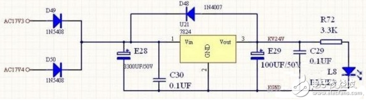
光电隔离电路设计方案(六款基于光耦、AD210AN的光电隔离电路图)

IJCAI 2022 outstanding papers were published, and 298 Chinese mainland authors won the first place in two items
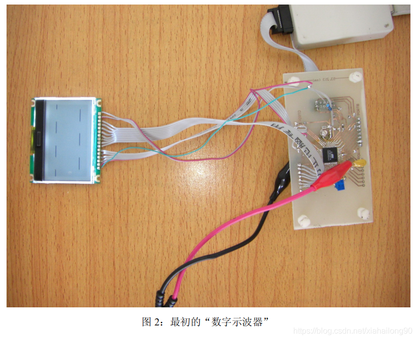
DIY制作示波器的超详细教程:(一)我不是为了做一个示波器

4种单片机驱动继电器方案
USB interface electromagnetic compatibility (EMC) solution

generic paradigm

JUC(JMM、Volatile)

随机推荐
"Sword finger offer" linked list inversion
Digital storage oscilloscope based on FIFO idt7202-12
Distributed lock
Network equipment hard core technology insider router Chapter 17 dpdk and its prequel (II)
网络设备硬核技术内幕 路由器篇 3 贾宝玉梦游太虚幻境 (中)
Sword finger offer cut rope
Some binary bit operations
TCC
USB接口电磁兼容(EMC)解决方案
How "Crazy" is Hefu Laomian, which is eager to be listed, with capital increasing frequently?
Method of removing top navigation bar in Huawei Hongmeng simulator
Overview of wechat public platform development
网络设备硬核技术内幕 路由器篇 7 汤普金森漫游网络世界(下)
How to edit a framework resource file separately
Deveco studio2.1 operation item error
JMeter recording interface automation
一些二进制位操作
Selenium 报错:session not created: This version of ChromeDriver only supports Chrome version 81
Network equipment hard core technology insider router Chapter 4 Jia Baoyu sleepwalking in Taixu Fantasy (Part 2)
Network equipment hard core technology insider router Chapter 9 Cisco asr9900 disassembly (II)