Opencv learning notes II

grayscale

import cv2 #opencv The reading format is BGR
import numpy as np
import matplotlib.pyplot as plt#Matplotlib yes RGB
%matplotlib inline 

img=cv2.imread('cat.jpg')
img_gray = cv2.cvtColor(img,cv2.COLOR_BGR2GRAY)
img_gray.shape

(414, 500)

cv2.imshow("img_gray", img_gray)
cv2.waitKey(0)    
cv2.destroyAllWindows() 

HSV

• H - tonal （ Main wavelength ）.
• S - saturation （ The purity / The shadow of color ）.
• V value （ Strength ）

hsv=cv2.cvtColor(img,cv2.COLOR_BGR2HSV)

cv2.imshow("hsv", hsv)
cv2.waitKey(0)    
cv2.destroyAllWindows()

b,g,r = cv2.split(hsv)
hsv_rgb = cv2.merge((r,g,b))
plt.imshow(hsv_rgb)
plt.show()

Image threshold

ret, dst = cv2.threshold(src, thresh, maxval, type)

• src： Input diagram , Only single channel images can be input , It's usually grayscale

• dst： Output chart

• thresh： threshold

• maxval： When the pixel value exceeds the threshold （ Or less than the threshold , according to type To decide ）, The value assigned to

• type： The type of binarization operation , Contains the following 5 Types ： cv2.THRESH_BINARY; cv2.THRESH_BINARY_INV; cv2.THRESH_TRUNC; cv2.THRESH_TOZERO;cv2.THRESH_TOZERO_INV

• cv2.THRESH_BINARY The part exceeding the threshold is taken as maxval（ Maximum ）, Otherwise take 0

• cv2.THRESH_BINARY_INV THRESH_BINARY The reversal of

• cv2.THRESH_TRUNC The part greater than the threshold is set as the threshold , Otherwise unchanged

• cv2.THRESH_TOZERO Parts larger than the threshold do not change , Otherwise, it is set to 0

• cv2.THRESH_TOZERO_INV THRESH_TOZERO The reversal of

ret, thresh1 = cv2.threshold(img_gray, 127, 255, cv2.THRESH_BINARY)
ret, thresh2 = cv2.threshold(img_gray, 127, 255, cv2.THRESH_BINARY_INV)
ret, thresh3 = cv2.threshold(img_gray, 127, 255, cv2.THRESH_TRUNC)
ret, thresh4 = cv2.threshold(img_gray, 127, 255, cv2.THRESH_TOZERO)
ret, thresh5 = cv2.threshold(img_gray, 127, 255, cv2.THRESH_TOZERO_INV)

titles = ['Original Image', 'BINARY', 'BINARY_INV', 'TRUNC', 'TOZERO', 'TOZERO_INV']
images = [img, thresh1, thresh2, thresh3, thresh4, thresh5]

for i in range(6):
    plt.subplot(2, 3, i + 1), plt.imshow(images[i], 'gray')
    plt.title(titles[i])
    plt.xticks([]), plt.yticks([])
plt.show()

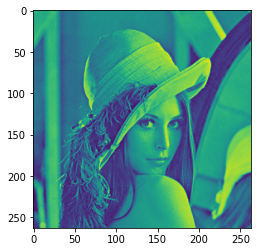
Image smoothing

img = cv2.imread('lenaNoise.png')

cv2.imshow('img', img)
cv2.waitKey(0)
cv2.destroyAllWindows()

b,g,r = cv2.split(img)
img_rgb = cv2.merge((r,g,b))
plt.imshow(img_rgb)
plt.show()

#  Mean filtering 
#  Simple average convolution operation 
blur = cv2.blur(img, (3, 3))

cv2.imshow('blur', blur)
cv2.waitKey(0)
cv2.destroyAllWindows()

b,g,r = cv2.split(blur)
blur_rgb = cv2.merge((r,g,b))
plt.imshow(blur_rgb)
plt.show()

#  Box filtering 
#  It's basically the same as the average , You can choose to normalize 
box = cv2.boxFilter(img,-1,(3,3), normalize=True)  #-1 Indicates that the number of color channels is consistent with the number of previously entered image color channels 

cv2.imshow('box', box)
cv2.waitKey(0)
cv2.destroyAllWindows()

b,g,r = cv2.split(box)
box_rgb = cv2.merge((r,g,b))
plt.imshow(box_rgb)
plt.show()

#  Box filtering 
#  It's basically the same as the average , You can choose to normalize , Easy to cross the border  , That is, the pixel value is greater than 255
box = cv2.boxFilter(img,-1,(3,3), normalize=False)  

cv2.imshow('box', box)
cv2.waitKey(0)
cv2.destroyAllWindows()

b,g,r = cv2.split(box)
box_rgb = cv2.merge((r,g,b))
plt.imshow(box_rgb)
plt.show()

#  Gauss filtering 
#  The values in the convolution kernel of Gaussian blur satisfy the Gaussian distribution , It's equivalent to paying more attention to the middle , That is, the weight of the middle pixel value of the core is relatively large 
aussian = cv2.GaussianBlur(img, (5, 5), 1)  

cv2.imshow('aussian', aussian)
cv2.waitKey(0)
cv2.destroyAllWindows()

b,g,r = cv2.split(aussian)
aussian_rgb = cv2.merge((r,g,b))
plt.imshow(aussian_rgb)
plt.show()

#  median filtering 
#  It's equivalent to using the median instead of 
median = cv2.medianBlur(img, 5)  #  median filtering 

cv2.imshow('median', median)
cv2.waitKey(0)
cv2.destroyAllWindows()

b,g,r = cv2.split(median)
median_rgb = cv2.merge((r,g,b))
plt.imshow(median_rgb)
plt.show()

#  Show all of them 
res = np.hstack((blur,aussian,median)) # They are stitched together horizontally 
#res = np.vstack((blur,aussian,median)) # Vertically spliced together 
#print (res)
cv2.imshow('median vs average', res)
cv2.waitKey(0)
cv2.destroyAllWindows()

b,g,r = cv2.split(res)
res_rgb = cv2.merge((r,g,b))
plt.imshow(res_rgb)
plt.show()

morphology - Corrosion operation

img = cv2.imread('cloudytosunny1.png')

cv2.imshow('img', img)
cv2.waitKey(0)
cv2.destroyAllWindows()

b,g,r = cv2.split(img)
img_rgb = cv2.merge((r,g,b))
plt.imshow(img_rgb)
plt.show()

kernel = np.ones((4,4),np.uint8) 
erosion = cv2.erode(img,kernel,iterations = 1)

cv2.imshow('erosion', erosion)
cv2.waitKey(0)
cv2.destroyAllWindows()

b,g,r = cv2.split(erosion)
erosion_rgb = cv2.merge((r,g,b))
plt.imshow(erosion_rgb)
plt.show()

pie = cv2.imread('pie.png')

cv2.imshow('pie', pie)
cv2.waitKey(0)
cv2.destroyAllWindows()

b,g,r = cv2.split(pie)
pie_rgb = cv2.merge((r,g,b))
plt.imshow(pie_rgb)
plt.show()

kernel = np.ones((30,30),np.uint8) 
erosion_1 = cv2.erode(pie,kernel,iterations = 1)
erosion_2 = cv2.erode(pie,kernel,iterations = 2)
erosion_3 = cv2.erode(pie,kernel,iterations = 3)
res = np.hstack((erosion_1,erosion_2,erosion_3))
cv2.imshow('res', res)
cv2.waitKey(0)
cv2.destroyAllWindows()

b,g,r = cv2.split(res)
res_rgb = cv2.merge((r,g,b))
plt.imshow(res_rgb)
plt.show()

morphology - Expansion operation

img = cv2.imread('cloudytosunny1.png')
cv2.imshow('img', img)
cv2.waitKey(0)
cv2.destroyAllWindows()

b,g,r = cv2.split(img)
img_rgb = cv2.merge((r,g,b))
plt.imshow(img_rgb)
plt.show()

kernel = np.ones((5,5),np.uint8) 
sunny_erosion = cv2.erode(img,kernel,iterations = 1)

cv2.imshow('erosion', sunny_erosion)
cv2.waitKey(0)
cv2.destroyAllWindows()

b,g,r = cv2.split(sunny_erosion)
sunny_erosion_rgb = cv2.merge((r,g,b))
plt.imshow(sunny_erosion_rgb)
plt.show()

kernel = np.ones((5,5),np.uint8) 
sunny_dilate = cv2.dilate(sunny_erosion,kernel,iterations = 1)

cv2.imshow('dilate', sunny_dilate)
cv2.waitKey(0)
cv2.destroyAllWindows()

b,g,r = cv2.split(sunny_dilate)
sunny_dilate_rgb = cv2.merge((r,g,b))
plt.imshow(sunny_dilate_rgb)
plt.show()

pie = cv2.imread('pie.png')

kernel = np.ones((30,30),np.uint8) 
dilate_1 = cv2.dilate(pie,kernel,iterations = 1)
dilate_2 = cv2.dilate(pie,kernel,iterations = 2)
dilate_3 = cv2.dilate(pie,kernel,iterations = 3)
res = np.hstack((dilate_1,dilate_2,dilate_3))
cv2.imshow('res', res)
cv2.waitKey(0)
cv2.destroyAllWindows()

b,g,r = cv2.split(res)
res_rgb = cv2.merge((r,g,b))
plt.imshow(res_rgb)
plt.show()

Open operation and closed operation

#  open ： Corrode first , Re expansion 
img = cv2.imread('cloudytosunny1.png')

kernel = np.ones((5,5),np.uint8) 
opening = cv2.morphologyEx(img, cv2.MORPH_OPEN, kernel)

cv2.imshow('opening', opening)
cv2.waitKey(0)
cv2.destroyAllWindows()

b,g,r = cv2.split(opening)
opening_rgb = cv2.merge((r,g,b))
plt.imshow(opening_rgb)
plt.show()

#  close ： Inflate first , Corrode again 
img = cv2.imread('cloudytosunny1.png')

kernel = np.ones((5,5),np.uint8) 
closing = cv2.morphologyEx(img, cv2.MORPH_CLOSE, kernel)

cv2.imshow('closing', closing)
cv2.waitKey(0)
cv2.destroyAllWindows()

b,g,r = cv2.split(closing)
closing_rgb = cv2.merge((r,g,b))
plt.imshow(closing_rgb)
plt.show()

Gradient operation

#  gradient = inflation - corrosion 
pie = cv2.imread('pie.png')
kernel = np.ones((7,7),np.uint8) 
dilate = cv2.dilate(pie,kernel,iterations = 5)
erosion = cv2.erode(pie,kernel,iterations = 5)

res = np.hstack((dilate,erosion))

b,g,r = cv2.split(res)
res_rgb = cv2.merge((r,g,b))
plt.imshow(res_rgb)
plt.show()

gradient = cv2.morphologyEx(pie, cv2.MORPH_GRADIENT, kernel)

b,g,r = cv2.split(gradient)
gradient_rgb = cv2.merge((r,g,b))
plt.imshow(gradient_rgb)
plt.show()

Hats and black hats

• formal hat = Raw input - The result of the open operation is
• Black hat = Closed operation - Raw input

# formal hat 
img = cv2.imread('cloudytosunny1.png')
tophat = cv2.morphologyEx(img, cv2.MORPH_TOPHAT, kernel)

b,g,r = cv2.split(tophat)
tophat_rgb = cv2.merge((r,g,b))
plt.imshow(tophat_rgb)
plt.show()

# Black hat 
img = cv2.imread('cloudytosunny1.png')
blackhat  = cv2.morphologyEx(img,cv2.MORPH_BLACKHAT, kernel)

b,g,r = cv2.split(blackhat)
blackhat_rgb = cv2.merge((r,g,b))
plt.imshow(blackhat_rgb)
plt.show()

Image gradient -Sobel operator

img = cv2.imread('pie.png',cv2.IMREAD_GRAYSCALE)

# b,g,r = cv2.split(img)
# img_rgb = cv2.merge((r,g,b))
plt.imshow(img)
plt.show()

cv2.imshow("img",img)
cv2.waitKey()
cv2.destroyAllWindows()

dst = cv2.Sobel(src, ddepth, dx, dy, ksize)

• ddepth: The depth of the image
• dx and dy Horizontal and vertical directions respectively
• ksize yes Sobel The size of the operator

def cv_show(img,name):
    b,g,r = cv2.split(img)
    img_rgb = cv2.merge((r,g,b))
    plt.imshow(img_rgb)
    plt.show()
def cv_show1(img,name):
    plt.imshow(img)
    plt.show()
    cv2.imshow(name,img)
    cv2.waitKey()
    cv2.destroyAllWindows()

sobelx = cv2.Sobel(img,cv2.CV_64F,1,0,ksize=3)

cv_show1(sobelx,'sobelx')

White to black is a positive number , Black to white is negative , All negative numbers are truncated to 0, So take the absolute value

sobelx = cv2.Sobel(img,cv2.CV_64F,1,0,ksize=3)
sobelx = cv2.convertScaleAbs(sobelx)
cv_show1(sobelx,'sobelx')

sobely = cv2.Sobel(img,cv2.CV_64F,0,1,ksize=3)
sobely = cv2.convertScaleAbs(sobely)  
cv_show1(sobely,'sobely')

Separate calculation x and y, And then sum up

sobelxy = cv2.addWeighted(sobelx,0.5,sobely,0.5,0)
cv_show1(sobelxy,'sobelxy')

Direct calculation is not recommended

sobelxy=cv2.Sobel(img,cv2.CV_64F,1,1,ksize=3)
sobelxy = cv2.convertScaleAbs(sobelxy) 
cv_show1(sobelxy,'sobelxy')

img = cv2.imread('lena.jpg',cv2.IMREAD_GRAYSCALE)
cv_show1(img,'img')

img = cv2.imread('lena.jpg',cv2.IMREAD_GRAYSCALE)
sobelx = cv2.Sobel(img,cv2.CV_64F,1,0,ksize=3)
sobelx = cv2.convertScaleAbs(sobelx)
sobely = cv2.Sobel(img,cv2.CV_64F,0,1,ksize=3)
sobely = cv2.convertScaleAbs(sobely)
sobelxy = cv2.addWeighted(sobelx,0.5,sobely,0.5,0)
cv_show1(sobelxy,'sobelxy')

img = cv2.imread(‘lena.jpg’,cv2.IMREAD_GRAYSCALE)

sobelxy=cv2.Sobel(img,cv2.CV_64F,1,1,ksize=3)
sobelxy = cv2.convertScaleAbs(sobelxy)
cv_show(sobelxy,‘sobelxy’)

Image gradient -Scharr operator

Image gradient -laplacian operator

# The difference between different operators 
img = cv2.imread('lena.jpg',cv2.IMREAD_GRAYSCALE)
sobelx = cv2.Sobel(img,cv2.CV_64F,1,0,ksize=3)
sobely = cv2.Sobel(img,cv2.CV_64F,0,1,ksize=3)
sobelx = cv2.convertScaleAbs(sobelx)   
sobely = cv2.convertScaleAbs(sobely)  
sobelxy =  cv2.addWeighted(sobelx,0.5,sobely,0.5,0)  

scharrx = cv2.Scharr(img,cv2.CV_64F,1,0)
scharry = cv2.Scharr(img,cv2.CV_64F,0,1)
scharrx = cv2.convertScaleAbs(scharrx)   
scharry = cv2.convertScaleAbs(scharry)  
scharrxy =  cv2.addWeighted(scharrx,0.5,scharry,0.5,0) 

laplacian = cv2.Laplacian(img,cv2.CV_64F) # It is not used alone , Will be used in conjunction with other methods 
laplacian = cv2.convertScaleAbs(laplacian)   

res = np.hstack((sobelxy,scharrxy,laplacian))
cv_show1(res,'res')

img = cv2.imread('lena.jpg',cv2.IMREAD_GRAYSCALE)
cv_show1(img,'img')

Canny edge detection

• 1.     Using a Gaussian filter , To smooth the image , Filter out noise .
     

• 2.     Calculate the gradient intensity and direction of each pixel in the image .
     

• 3.     Apply non maxima （Non-Maximum Suppression） Inhibition , To eliminate the spurious response brought by edge detection .
     

• 4.     Apply double thresholds （Double-Threshold） Detection to determine real and potential edges .
     

• 5.     Finally, the edge detection is completed by suppressing the isolated weak edge .
     

1: Gauss filter

2: Gradient and direction

3： Non maximum suppression

4： Double threshold detection

img=cv2.imread("lena.jpg",cv2.IMREAD_GRAYSCALE)

v1=cv2.Canny(img,80,150)
v2=cv2.Canny(img,50,100)

res = np.hstack((v1,v2))
cv_show1(res,'res')

img=cv2.imread("car.png",cv2.IMREAD_GRAYSCALE)

v1=cv2.Canny(img,120,250)
v2=cv2.Canny(img,50,100)

res = np.hstack((v1,v2))
cv_show1(res,'res')

Image pyramid

• The pyramid of Gauss
• The pyramid of Laplace

The pyramid of Gauss ： Down sampling method （ narrow ）

The pyramid of Gauss ： Up sampling method （ Zoom in ）

img=cv2.imread("AM.png")
cv_show(img,'img')
print (img.shape)

(442, 340, 3)

up=cv2.pyrUp(img)
cv_show(up,'up')
print (up.shape)

(884, 680, 3)

down=cv2.pyrDown(img)
cv_show(down,'down')
print (down.shape)

(221, 170, 3)

up2=cv2.pyrUp(up)
cv_show(up2,'up2')
print (up2.shape)

(1768, 1360, 3)

up=cv2.pyrUp(img)
up_down=cv2.pyrDown(up)
cv_show(up_down,'up_down')

cv_show(np.hstack((img,up_down)),'up_down')

up=cv2.pyrUp(img)
up_down=cv2.pyrDown(up)
cv_show(img-up_down,'img-up_down')

The pyramid of Laplace

down=cv2.pyrDown(img)
down_up=cv2.pyrUp(down)
l_1=img-down_up
cv_show(l_1,'l_1')

Image outline

cv2.findContours(img,mode,method)

mode: Contour retrieval mode

• RETR_EXTERNAL ： Retrieve only the outermost outline ;
• RETR_LIST： Retrieve all the contours , And save it in a linked list ;
• RETR_CCOMP： Retrieve all the contours , And organize them into two layers ： The top layer is the outer boundary of the parts , The second layer is the boundary of the void ;
• RETR_TREE： Retrieve all the contours , And reconstruct the entire hierarchy of nested profiles ;

method: Contour approximation method

• CHAIN_APPROX_NONE： With Freeman Chain code output outline , All other methods output polygons （ The sequence of vertices ）.
• CHAIN_APPROX_SIMPLE: Compressed horizontal 、 The vertical and oblique parts , That is to say , Functions keep only the end part of them .

For higher accuracy , Use binary images .

img = cv2.imread('contours.png')
gray = cv2.cvtColor(img, cv2.COLOR_BGR2GRAY)
ret, thresh = cv2.threshold(gray, 127, 255, cv2.THRESH_BINARY)
cv_show1(thresh,'thresh')

binary, contours, hierarchy = cv2.findContours(thresh, cv2.RETR_TREE, cv2.CHAIN_APPROX_NONE)

Draw the outline

cv_show(img,'img')

# Pass in the drawing image , outline , Outline index , Color mode , Line thickness 
#  Pay attention to the need for copy, Or the original picture will change ...
draw_img = img.copy()
res = cv2.drawContours(draw_img, contours, -1, (0, 0, 255), 2)
cv_show(res,'res')

draw_img = img.copy()
res = cv2.drawContours(draw_img, contours, 0, (0, 0, 255), 2)
cv_show(res,'res')

Contour feature

cnt = contours[0]

# area 
cv2.contourArea(cnt)

8500.5

# Perimeter ,True It means closed 
cv2.arcLength(cnt,True)

437.9482651948929

The outline is approximate

img = cv2.imread('contours2.png')

gray = cv2.cvtColor(img, cv2.COLOR_BGR2GRAY)
ret, thresh = cv2.threshold(gray, 127, 255, cv2.THRESH_BINARY)
binary, contours, hierarchy = cv2.findContours(thresh, cv2.RETR_TREE, cv2.CHAIN_APPROX_NONE)
cnt = contours[0]

draw_img = img.copy()
res = cv2.drawContours(draw_img, [cnt], -1, (0, 0, 255), 2)
cv_show(res,'res')

epsilon = 0.1*cv2.arcLength(cnt,True) 
approx = cv2.approxPolyDP(cnt,epsilon,True)

draw_img = img.copy()
res = cv2.drawContours(draw_img, [approx], -1, (0, 0, 255), 2)
cv_show(res,'res')

Border rectangle

img = cv2.imread('contours.png')

gray = cv2.cvtColor(img, cv2.COLOR_BGR2GRAY)
ret, thresh = cv2.threshold(gray, 127, 255, cv2.THRESH_BINARY)
binary, contours, hierarchy = cv2.findContours(thresh, cv2.RETR_TREE, cv2.CHAIN_APPROX_NONE)
cnt = contours[0]

x,y,w,h = cv2.boundingRect(cnt)
img = cv2.rectangle(img,(x,y),(x+w,y+h),(0,255,0),2)
cv_show(img,'img')

area = cv2.contourArea(cnt)
x, y, w, h = cv2.boundingRect(cnt)
rect_area = w * h
extent = float(area) / rect_area
print (' The ratio of contour area to boundary rectangle ',extent)

 The ratio of contour area to boundary rectangle  0.5154317244724715

Circumcircle

(x,y),radius = cv2.minEnclosingCircle(cnt) 
center = (int(x),int(y)) 
radius = int(radius) 
img = cv2.circle(img,center,radius,(0,255,0),2)
cv_show(img,'img')

The Fourier transform

We live in a world of time , morning 7:00 Get up for breakfast ,8:00 To squeeze the subway ,9:00 Start to work ... Time reference is time domain analysis .

But in the frequency domain everything is still ！

https://zhuanlan.zhihu.com/p/19763358

The role of Fourier transform

• high frequency ： The grayscale components that change dramatically , For example, borders

• Low frequency ： Slowly changing gray components , For example, a sea

wave filtering

• low pass filter ： Keep only the low frequencies , It will blur the image

• High pass filter ： Keep only the high frequencies , Will enhance the image details

• opencv The main thing is cv2.dft() and cv2.idft(), The input image needs to be converted into np.float32 Format .

• The frequency of the result is 0 It's going to be in the upper left corner , It's usually a shift to a central position , Can pass shift Transform to achieve .

• cv2.dft() The result returned is dual channel （ Real component , Imaginary part ）, Usually it needs to be converted to image format to display （0,255）.

import numpy as np
import cv2
from matplotlib import pyplot as plt

img = cv2.imread('lena.jpg',0)

img_float32 = np.float32(img)

dft = cv2.dft(img_float32, flags = cv2.DFT_COMPLEX_OUTPUT)
dft_shift = np.fft.fftshift(dft)
#  Get the form that the gray image can express 
magnitude_spectrum = 20*np.log(cv2.magnitude(dft_shift[:,:,0],dft_shift[:,:,1]))

plt.subplot(121),plt.imshow(img, cmap = 'gray')
plt.title('Input Image'), plt.xticks([]), plt.yticks([])
plt.subplot(122),plt.imshow(magnitude_spectrum, cmap = 'gray')
plt.title('Magnitude Spectrum'), plt.xticks([]), plt.yticks([])
plt.show()

import numpy as np
import cv2
from matplotlib import pyplot as plt

img = cv2.imread('lena.jpg',0)

img_float32 = np.float32(img)

dft = cv2.dft(img_float32, flags = cv2.DFT_COMPLEX_OUTPUT)
dft_shift = np.fft.fftshift(dft)

rows, cols = img.shape
crow, ccol = int(rows/2) , int(cols/2)     #  Center position 

#  Low pass filtering 
mask = np.zeros((rows, cols, 2), np.uint8)
mask[crow-30:crow+30, ccol-30:ccol+30] = 1

# IDFT
fshift = dft_shift*mask
f_ishift = np.fft.ifftshift(fshift)
img_back = cv2.idft(f_ishift)
img_back = cv2.magnitude(img_back[:,:,0],img_back[:,:,1])

plt.subplot(121),plt.imshow(img, cmap = 'gray')
plt.title('Input Image'), plt.xticks([]), plt.yticks([])
plt.subplot(122),plt.imshow(img_back, cmap = 'gray')
plt.title('Result'), plt.xticks([]), plt.yticks([])

plt.show()                

img = cv2.imread('lena.jpg',0)

img_float32 = np.float32(img)

dft = cv2.dft(img_float32, flags = cv2.DFT_COMPLEX_OUTPUT)
dft_shift = np.fft.fftshift(dft)

rows, cols = img.shape
crow, ccol = int(rows/2) , int(cols/2)     #  Center position 

#  High pass filtering 
mask = np.ones((rows, cols, 2), np.uint8)
mask[crow-30:crow+30, ccol-30:ccol+30] = 0

# IDFT
fshift = dft_shift*mask
f_ishift = np.fft.ifftshift(fshift)
img_back = cv2.idft(f_ishift)
img_back = cv2.magnitude(img_back[:,:,0],img_back[:,:,1])

plt.subplot(121),plt.imshow(img, cmap = 'gray')
plt.title('Input Image'), plt.xticks([]), plt.yticks([])
plt.subplot(122),plt.imshow(img_back, cmap = 'gray')
plt.title('Result'), plt.xticks([]), plt.yticks([])

plt.show()