2021-02-27image processing of MATLAB

The image processing

imread

I=imread("path")

I It becomes a picture unit

imshow(I)

display picture
Original size 、 Borderless display ：

imshow(i,'border','tight')

imshow(I,[low high])

Less than low It's black 、 Greater than high It's white , It should mean , Set a threshold to prevent overflow , If it is [],low、high Is the minimum and maximum
If you specify an empty matrix ([]), then imshow uses a display range of [min(I() max(I()]

size(I)

Size
We can find that the output of the color map is Long wide 3（rgb Tricolor ）

imresize

i=imresize(i,[m,n]);
Resize the image

Image conversion function

• gray2ind(I,8) - intensity image to index image
• im2bw(I,0.5) - image to binary
• im2double - image to double precision
• im2uint8 - image to 8-bit unsigned integers
• im2uint16 - image to 16-bit unsigned integers
• ind2gray - indexed image to intensity image
• mat2gray - matrix to intensity image
• rgb2gray - RGB image to grayscale
• rgb2ind - RGB image to indexed image

im=image picture
gray=intensity Intensity diagram , The grayscale is 256 Bit intensity diagram （ Can that be understood ）
bw=binary It's a binary graph , A threshold value is required in the parameter （0-1 representative 0-256）
ind=index

Image addition

In order to preserve the accuracy, the addition of images needs to be transformed into double

mI=uint8(double(I1)+double(I2)+double(I3));

A1 = imread('rice.png');
A2 = imread('cameraman.tif');
K = imadd(A1,A2,'uint16');% Image addition , Prevent pixel values from exceeding 255, So save the result as 16 position 
%K = imlincomb(0.5,A1,0.5,A2);  Used to adjust the scale of addition 
figure;
subplot(1,3,1);imshow(A1);title('rice original image ');
subplot(1,3,2);imshow(A2);title('cameraman original image ');
subplot(1,3,3);imshow(K,[]);title(' Additive image ');% Pay attention to imshow Function time , To add [], So that the pixel value is compressed to 0—255

Image segmentation

mat2cell

mat2cell(i,[x1,x2,…],[y1,y2,…],…） How many dimensions are there , How many vectors are there , At the same time, the sum of the elements in the vector and the value of that dimension should be equal , So before using, adjust the size of the picture to an integer multiple of the size to be cut .

Intensity conversion

>> aI2=imadjust(I0,[],[],0.5);

>> aI1=imadjust(I0,[0,1],[1,0]);

The first line of code adjusts the intensity of the image through the following parameters , The default is 1, This is a linear mapping

The middle two parameters represent
[low_in;high_in],[low_out;high_out]

Indicates the range of gray scale before and after conversion

Statistical histogram

Statistics of color distribution

imhist(I0)

Image cropping

b = imcrop(I,[403,0,810,1080]);

Image opening and closing operation

Anyway, corrosion is less white , Expansion is the increase of whiteness
It is considered as corrosion before expansion , Used to eliminate small objects ; Closed operation is to expand first and then corrode , Used to connect small gaps .

i=imread('image.jpg');
i1=rgb2gray(i); % Grayscale image 
i2=im2bw(i1);    % Binary search 
i3 = bwmorph(i2,'close');  % Closed operation 
imshow(i3)
i4 = bwmorph(i2,'open');  % Open operation 
figure, imshow(i4)

Image rotation and distortion

Using affine plus twist function , Commonly used to enhance image data

tform = affine2d([1 0 0; .5 1 0; 0 0 1])
J = imwarp(I,tform);
figure
imshow(J)

I = imread('kobi.png');
imshow(I)
tform1 = randomAffine2d('Rotation',[35 55]);% stay 35° and 55° Random rotation between 
J = imwarp(I,tform1);
imshow(J)

Image zoom

Nearest neighbor resampling

Find the nearest one to interpolate , There will be a lot of noise

Bilinear interpolation

Maintain the interpolation of the two dimensions

I=imread('pic1.png');
I=I0;
I0=double(I0);
I1=zeros(size(I0,1)*2,size(I0,2)*2,3);
[r,c]=meshgrid(1:size(I0,2),1:size(I0,1));
rc=linspace(1, size(I,1), size(I,1)*2);
cc=linspace(1, size(I,2), size(I,2)*2);
[r_new,c_new]=meshgrid(cc,rc);
rc=linspace(1, size(I0,1), size(I0,1)*2);
cc=linspace(1, size(I0,2), size(I0,2)*2);
[r_new,c_new]=meshgrid(cc,rc);
I1(:,:,1)=interp2(r,c,I0(:,:,1),r_new,c_new,'spline');
I1(:,:,2)=interp2(r,c,I0(:,:,2),r_new,c_new,'spline');
I1(:,:,3)=interp2(r,c,I0(:,:,3),r_new,c_new,'spline');
imshow(uint8(I1))
size(I1)

interp2 Is a bilinear interpolation function
If the magnification is a fraction , The size is written like this round(size(I0,1)*p/q)

Image denoising

The noise contains white Gaussian noise 、 Salt and pepper noise

Add noise

nI = imnoise(I0, 'gaussian', 0, 0.01);
nI = imnoise(I0, ‘salt & pepper', 0.01);

Gaussian noise and salt and pepper noise

I0=imread('pic3.png');
I0(100:105,800:808,:)=0;
figure,imshow(I0)

Addition of outliers

Noise reduction 、 wave filtering

Nonlinear filtering and noise reduction ： median filtering

k=medfilt2(spl,[5,5]);

Incoming picture and filter operator size , The image should be grayscale

The filter operator defaults to 3*3

filt： filter

Baidu for more filters

The use of filters , Edge detection

The principle of the filter is a convolution operation between the characteristic matrix and the image （ Equivalent to sliding on the surface of the image , If noise is detected , Will keep ）

Abnormal point detection

Point detection operator

-1 -1 -1
-1  8 -1
-1 -1 -1

 w=[-1 -1 -1;-1 8 -1;-1 -1 -1]
g=abs(imfilter(I0,w));
T=max(g(:));
g=(g>=T);
imshow(uint8(g))

Straight line detection

Horizontal line detection operator

-1 -1 -1
 2  2  2
-1 -1 -1

Others in the same way , But there are too few kinds of straight lines that can be detected

Edge detector

Commonly used canny operator

I=imread('pic4.png');
I0=rgb2gray(I);
subplot(231);
imshow(I);

BW1=edge(I0,'Roberts',0.16);
subplot(232);
imshow(BW1);
title('Roberts')


BW2=edge(I0,'Sobel',0.16);
subplot(233);
imshow(BW2);
title('Sobel')

BW3=edge(I0,'Prewitt',0.16);
subplot(234);
imshow(BW3);
title('Prewitt');

BW4=edge(I0,'LOG',0.012);
subplot(235);
imshow(BW4);
title('LOG')

BW5=edge(I0,'Canny',0.2);
subplot(236);
imshow(BW5);
title('Canny');

Add text to picture

text function

Feeling MATLAB The function of is amazing , Below text Add dimensions to

x = 0:pi/20:2*pi;
y = sin(x);
plot(x,y)
text(pi,0,'\leftarrow sin(\pi)')

\leftarrow Is the left arrow ,pi 0 Such a point can be changed into a vector , Represents a multipoint dimension
The results are as follows

plot(1:10)
str = {
    {
    'A simple plot','from 1 to 10'},'y = x'};
text([2 8],[7 7],str)

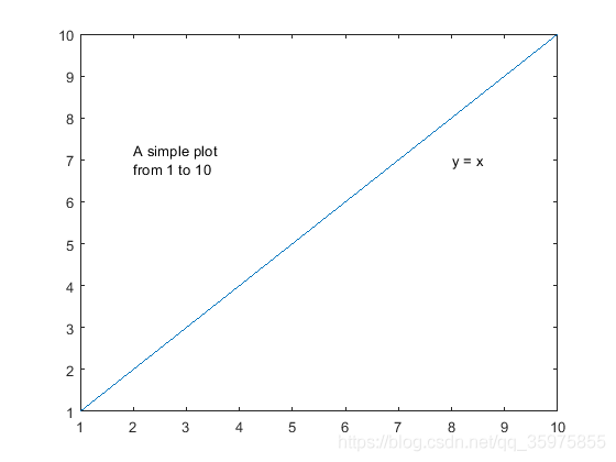
It is worth noting that , use text Not only can you write words , You can also draw spot 、 asterisk Wait for the pattern .

getframe function

This function is used to intercept the state of the window （ Screenshot ）, Achieve the effect of writing on the picture

 F = getframe(figure(1));
 figure(2)
 imshow(F.cdata)

Digression ：getframe Related animation production

[X, Y, Z] = peaks(30);  
% surf Draw a three-dimensional surface   
surf(X,Y,Z);  
   
axis([-3,3,-3,3,-10,10]);  
%  Close the mark on the coordinate axis used 、 Grating and unit marking . But reserved by text and gtext Set object   
axis off;  
shading interp;   
colormap(hot);  

M = moviein(20);%  Build a 20 Large matrix of columns     
for i = 1:20    
   view(-37.5+24*(i-1),30);%  Change viewpoint      
   M(i) = getframe;%  Save the drawing to M matrix    
end  

movie(M,2);%  Play picture 2 Time 

Reference links for animation ：https://blog.csdn.net/qq_32892383/article/details/79553001

Add a box to the picture 、 rectangular

rectangle('Position',[100 100 100 100],'LineWidth',4,'EdgeColor','r');

The four coordinates of the vector are the coordinates of the top left corner vertex and the length and width of the matrix

Adjust the parameters to draw a solid rectangle

rectangle('Position',[1,2,5,10],'FaceColor','w','EdgeColor','w',...
    'LineWidth',3)

You can even draw rounded rectangles and circles

rectangle('Position',[3 0 2 4],'Curvature',1)

pos = [2 4 2 2]; 
rectangle('Position',pos,'Curvature',[1 1])
axis equal

Draw a grid on the picture

p = imread('path'); % Read images 
[mm,nn,~] = size(p); % Gets the size of the image 
x = 0:nn/10:nn; % Suppose the level is divided into 10 grid 
y = 0:mm/20:mm; % Let's say we split it vertically 20 grid 
M = meshgrid(x,y); % Generating grids 
N = meshgrid(y,x); % Generating grids 
imshow(p); % First draw the original picture 
hold on % Keep the original picture , As a canvas, add a grid on it 
plot(x,N,'y'); % Draw a horizontal line . there 'y' The color of the line is yellow 
%plot(M,y,'r'); % Draw a vertical line .'r' Indicates green red 

Draw... On the original

This method may not require getframe function , Operate directly on the original drawing

I = imread('peppers.png');
RGB = insertShape(I,'circle',[150 280 35],'LineWidth',5);
pos_triangle = [183 297 302 250 316 297];
pos_hexagon = [340 163 305 186 303 257 334 294 362 255 361 191];
RGB = insertShape(RGB,'FilledPolygon',{
    pos_triangle,pos_hexagon},...
    'Color', {
    'white','green'},'Opacity',0.7);
imshow(RGB);