[datawhale202206] pytorch recommendation system: precision model deepfm & DIN

Summary

The relevant background knowledge of the recommendation system is supplemented , It can better understand the two models learned this time ：DeepFM and DIN Role in Recommendation System （ Fine discharge ）.

Then I learned DeepFM and DIN The structure of the two models , Understanding the birth background of the model may be more noteworthy .

DeepFM The big background of trying to make the model is to learn more features , To improve the effect of the recommended model , The innovation lies in parallel processing FM and DNN, Make the high-level and low-level features better combined and learned ;

DIN The big background of is in the application scenario that has accumulated enough historical user behavior data , The innovation is the introduction of attention mechanism to deal with historical user behavior data . stay DIN in , Because the general background is different from the task of the conventional recommendation system （ There are a lot of historical user behavior data ）, Therefore, it is necessary to understand how historical user behavior data is represented in model input , And how to deal with it in the model and code implementation （ They are not equal in length -》multi-hot Equal length -》 The input model is not equal in length after it is dense -》 When the code is implemented padding Equal length ,mask Mark ）

0 rechub And recommendation systems

0.1 rechub Project and installation

rechub It is a practical recommendation model focusing on reproduction in the industry , And pan ecological recommended scenario projects , The goal is easy to use and expand , Project address

You can install through the following instructions

# Stable version  
pip install torch-rechub

# The latest version （ recommend ）
1. git clone https://github.com/datawhalechina/torch-rechub.git
2. cd torch-rechub
3. python setup.py install

This time at colab Configure the environment on , The implementation is as follows ：

The project homepage provides a more detailed introduction and simple examples of use .

0.2 Recommendation system

0.2.1 What is the recommendation system

stay Introduction to recommender system This blog has a very good brief introduction .

Recommender system is a kind of Information filtering system , According to the user's historical behavior 、 social connections 、 The interest point algorithm can determine the items or contents that users are currently interested in . You can also understand it as a store that only opens for you . What you need is displayed in the shop , Or suitable for your products .

The ways to implement recommendations are divided into ：

• Content-based Filtering： Label the content , Recommend other similar content
• Collaborative Filtering： Tag users , Recommend according to the behavior of similar users
• Using data to solve problems： With data , It is still divided into two aspects: content and user behavior , analysis data Judge the similarity , Then recommend solve problems

• Object itself ：Content-based Based on the content of the item itself , Instead of users buying / The act of browsing objects
• User behavior ：
  Explicit feedback data ： Users clearly express their preference for items ： score , like , Collection , Buy
  Implicit feedback data ： Behavior that does not clearly reflect user preferences ： Browse , residence time , Click on

0.2.2 Recommend the algorithm framework of the system

Because the main project involved is the algorithm model of the recommendation system , So we need to be familiar with the algorithm architecture of the recommendation system , from Recall , Rough row , Sort , rearrangement And other four algorithm links , The following figure is a simple illustration .

Correspondingly , The functions of the four algorithm links can be simply understood as ：

• Recall ： It can be understood as a process of quickly screening and forming noteworthy data , Specifically, tens of thousands of... Are selected from the recommendation pool item, Send it to the subsequent sorting module ;
• Rough row ： It can be understood as preliminary filtration calculation , Realize the process of reducing the calculation amount of fine arrangement layer ;
• Fine discharge ： Get the result of rough sorting module , Score and sort candidate sets . Fine scheduling is required when the maximum delay is allowed , Ensure the accuracy of scoring , It is a crucial module in the whole system , It's also the most complicated , The most studied module . The construction of fine-tuning system generally involves samples 、 features 、 The model consists of three parts ;
• rearrangement ： According to the specific purpose of use , Fine tune the result of fine-tuning ;
• Mixed platoon ： If there are multiple data sources , Here is a combination .

among , For the material warehouse mentioned in the above figure , Obviously, it will not be implemented in the form of an original accumulation of all data , Instead, it is organized into descriptions （ user / goods ） The data form of the portrait . Generally, the recommendation system will also add a content understanding of multimodality （ Including text understanding , Keyword tags , Content understanding , Knowledge map, etc ）.

The following figure shows the content portrait framework of wechat , It can help understand what is in the material warehouse , So we can have an understanding of the data that we need to process in our recommended algorithm .

The following passage can help us better understand the role of recommendation algorithm in actual recommendation system , And what we need to pay attention to .

When we are learning the recommendation system at the beginning , Which model is more concerned AUC Higher 、topK The effect is good , Which model is more awesome , From basic collaborative filtering to hit rate estimation algorithm , From deep learning to intensive learning , Academia has always been at the forefront . It is a long-term process from the emergence of a recommendation algorithm to its wide application in the industry , Because in the actual production system , The first thing we need to ensure is stability 、 Provide recommendation services to users in real time , Under this premise, we can pursue the effect of the recommendation system .
The design idea of algorithm architecture is in the actual industrial scene , Whether it's the user dimension 、 The item dimension is also the interaction dimension between users and items , The data is extremely rich , The use of algorithms in academia cannot be copied to industry . When a user accesses the recommendation module , The system cannot sort all items for this user , So how does the recommendation system solve it ？ There are many corresponding commodities , How to decide which products to show to users ？ For the sorted products , How to reasonably show it to users ？
So a general algorithm architecture , The design idea is Model the data layer by layer , Layer by layer screening , Help users find out what they are really interested in from the massive data .

in other words , For the actual recommendation system , It is not just necessary to make a simple recommendation algorithm model , Because it will be limited and affected by the quality, quantity and scale of data sources . therefore , Consider using a reasonable algorithm architecture , Filter data , Then maximize the effect of the algorithm model .

And what is involved this time , yes Fine discharge Link model .

Fine arrangement layer , It is also the layer we most often contact when learning to recommend , A large part of the algorithms we are familiar with come from the fine arrangement layer . The task of this layer is to obtain the results of rough sorting modules , Score and sort candidate sets . Fine scheduling is required when the maximum delay is allowed , Ensure the accuracy of scoring , It is a crucial module in the whole system , It's also the most complicated , The most studied module .
Fine tuning is the purest layer in the recommendation system , His goal is single and focused , Just focus on the tuning of the goal . In the beginning, the common goal of fine-tuning model is ctr, Later, it gradually developed cvr And so on . The basic goals of fine and coarse rows are the same , It is to sort the product collection , But different from the rough row , Fine sorting requires only a small amount of goods ( That is, the product set of rough output topN) Just sort it out . therefore , More features can be used in fine sorting than in coarse sorting , More complex models and more sophisticated strategies （ This is also the reason why users' characteristics and behaviors are widely used and participated in this layer ）.
The fine arrangement layer model is the most research direction covered in the recommendation system , There are many sub fields worth studying and exploring , This is also the most technical part of the recommendation system , After all, it is directly facing the user , The layer that produces the most impact on users . At present, the deep learning of fine arrangement layer has dominated the world , The scheme adopted in the fine arrangement stage is relatively general , First of all, the sample size of a day is several billion , What we need to solve is the problem of sample size , Feed the model as much as possible to remember , On the other hand, timeliness , When user feedback is generated , How to give new feedback to the model as soon as possible , Learn the latest knowledge .

0.2.3 Recommend the evaluation criteria of the system

According to the purpose , The recommendation system obviously has practical evaluation criteria , When the definition of evaluation objectives changes , The recommendation results will also change .

The evaluation objectives include but are not limited to the following figure （ source Introduction to recommender system ）：

• Accuracy ： Scoring system ,top N recommend
• coverage ： The ability to explore the long tail of objects
• diversity ： The dissimilarity between two items in the recommendation list
• Novelty ： To the user suprise
• Surprise degree ： Recommendations are not similar to users' historical interests , But satisfied
• Trust degree ： Provide reliable reasons for recommendation
• The real time ： Real time update degree

Specific to the evaluation criteria , Examples include

• CTR： Click through rate （ Clicks / The amount of display ）
• CVR： Transformation , Indicators concerned by businesses （ Conversion amount / Clicks ）
• GPM： Average 1000 Show , Average transaction amount
• etc.
  Choose according to the needs of the scene . Lots of scenes , Include （ source Introduction to recommender system ）：
  
  The models involved this time , Are facing CTR（ Click through rate ） Model of .

1 DeepFM

1.1 The background of the birth of the model

about CTR problem , The most effective strategy proved to improve task performance is feature combination (Feature Interaction), stay CTR Historically, the exploration of the problem is how to better learn the combination of features , And then describe the characteristics of data more accurately .

obviously , With the increase of feature combination , It will lead to an explosion of model complexity , So as to slow down the calculation speed . There is also a very important requirement for the practical application of the recommendation system The real time , therefore “ How to learn feature combination efficiently ” Become a very important issue .

DNN Is a good way to solve this problem , But there are limitations ： need Reasonably handle the expression form of features , To prevent the dimension from soaring , On this basis, increase the number of layers , Can achieve High order feature combination , But still Lack of low-order feature combination .

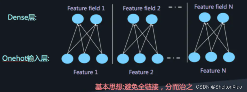
When we use DNN When the network solves the recommendation problem, there is a problem that the network parameters are too large , This is because we need to use one-hot Coding to deal with discrete features , This will cause the dimension of input to soar . Borrow here AI A picture of the Conference ：

Such a large number of parameters is also unrealistic . In order to solve DNN Limitations of excessive parameter quantity , You can use very classic Field thought , take OneHot The feature is transformed into Dense Vector

At this time, high-order feature combination can be achieved by adding a full connection layer , As shown in the figure below ：

But there is still a lack of low-order feature combinations .

At this time in DNN Introduction in FM To represent the low-order feature combination , There is FNN（ Serial FM and DNN）, and PNN（ stay FNN On the basis of, another product layer ）.

combination FM and DNN There are actually two ways , It can be combined in parallel or in serial . These two methods have several representative models . stay DeepFM Before a FNN, Although it may not be as influential as DeepFM, But understand FNN Our thoughts are understood by us DeepFM Its features and advantages are very helpful .

FNN It is pre trained FM modular , We get the hidden vector , Then take the hidden vector as DNN The input of , But after experiments, it was further found that , stay Embedding layer and hidden layer1 Add a product layer （ As shown in the figure above ） It can improve the performance of the model , So I put forward PNN, Use product layer Replace FM Pre training layer .

But the above model is directly serialized FM and DNN, The learning of low-order features is still not enough , So it evolved Wide&Deep Model （ Change the string behavior to parallel ）, from google Put forward （ For details, please refer to course ）.

FNN and PNN The model still has an obvious unresolved shortcoming ： Little is learned about low-order combined features , This is mainly due to FM and DNN Caused by the serial mode of , That is, although FM Learned low-order feature combination , however DNN The fully connected structure of leads to the fact that the low-order features cannot be in DNN Better performance of the output terminal .
Improving serial mode to parallel mode can better solve this problem . therefore Google Put forward Wide&Deep Model , But if you delve deeper Wide&Deep It's a way to make it up , Although the structure of the whole model is adjusted to parallel structure , In actual use Wide Module Some parts of the need for more sophisticated Feature Engineering , In other words, manual processing has a great impact on the effect of the model （ This can be found in Wide&Deep The model part is verified ）.

however , Simple parallel combination still has problems , Mainly limited by the combination form of features ：
stay output Units Stage directly combines low-order and high-order features , It is easy for the model to eventually learn low-order or high-order features , And can't do a good combination .

DeepFM It was born in this context , It tries to solve the problem of good combination of high-order and low-order .

1.2 Structure of model （ Thinking questions 2）

First lay out a model diagram

among ： Ahead Field and Embedding The processing is the same as the previous method , As shown in the green part in the above figure ;DeepFM take Wide Partially replaced with FM layer Like the blue part in the picture above

In the tutorial, we are reminded that there are three points to pay attention to in the model ：

• Deep The model part
  Deep Module In order to learn high-order feature combination , Use full connection to connect Dense Embedding Input to Hidden Layer, Inside this Dense Embeddings Just to solve it DNN The problem of parameter explosion in , This is also a common method in recommendation model .Embedding The output of the layer is to put all id Class features correspond to embedding vector concat Come together and type in DNN in .
  

• FM The model part
  FM Layer It is composed of first-order features and second-order features Concatenate Together after a Sigmoid obtain logits. We need to consider separately when implementing .
  

• Sparse Feature What do the yellow and gray nodes mean 【 Thinking questions 2】
  stay DeepFM In the structure diagram of the model ,Sparse Features The Yellow node in is connected to the model , Participated in training , The grey node did not participate in the training .
  According to the original paper , The Yellow node indicates that the value in the input sparse vector is 1 The point of , The value represented by grey nodes is 0 The point of , Because the value 0 The weight learned in the input model is still zero , So it can be regarded as not participating in training .
  （Sparse Feature All for need dense The discrete characteristics of （ Category features ））

1.3 Code implementation of the model

rechub Implemented in the DeepFM Model , The overall model architecture is as follows ：

The model consists of two parts

• FM（ It is further subdivided into the processing of first-order features and the processing of second-order features ）
• DNN
  Therefore, the implementation is refined into
• FM Linear feature processing
• FM Second order feature cross processing of
• DNN The higher order features of the intersection

This structure can also be clearly seen in the code . In addition, each part may be made up of different features , So when building the model, we need to select the input features of these three parts .

The code is as follows , For more detailed code, see GitHub

def DeepFM(linear_feature_columns, dnn_feature_columns):
    #  Build the input layer , That is, all features correspond to Input() layer , Here we use the form of a dictionary to return , Facilitate the subsequent construction of the model 
    dense_input_dict, sparse_input_dict = build_input_layers(linear_feature_columns + dnn_feature_columns)

    #  take linear Some of the features sparse Feature selection , The back is used to do 1 Dimensional embedding
    linear_sparse_feature_columns = list(filter(lambda x: isinstance(x, SparseFeat), linear_feature_columns))

    #  Build the input layer of the model , The input layer of the model cannot be in the form of a dictionary , You should convert the dictionary form to the list form 
    #  Be careful ： The actual input here is related to Input() Correspondence of layers , The dictionary data is input through the model key Corresponding to name Of Input layer 
    input_layers = list(dense_input_dict.values()) + list(sparse_input_dict.values())

    # linear_logits It's made up of two parts , Namely dense The characteristics of the logits and sparse The characteristics of the logits
    linear_logits = get_linear_logits(dense_input_dict, sparse_input_dict, linear_sparse_feature_columns)

    #  The construction dimension is k Of embedding layer , Here we use the form of a dictionary to return , It's convenient to build models in the back 
    # embedding Layer user building FM Cross section and DNN The input part of 
    embedding_layers = build_embedding_layers(dnn_feature_columns, sparse_input_dict, is_linear=False)

    #  Input to dnn All in sparse Feature selection 
    dnn_sparse_feature_columns = list(filter(lambda x: isinstance(x, SparseFeat), dnn_feature_columns))

    fm_logits = get_fm_logits(sparse_input_dict, dnn_sparse_feature_columns, embedding_layers) #  Consider only the second order term 

    #  Will all Embedding Put it all together , Input to dnn in 
    dnn_logits = get_dnn_logits(sparse_input_dict, dnn_sparse_feature_columns, embedding_layers)
    
    #  take linear,FM,dnn Of logits Add as the final logits
    output_logits = Add()([linear_logits, fm_logits, dnn_logits])

    #  The activation function here uses sigmoid
    output_layers = Activation("sigmoid")(output_logits)

    model = Model(input_layers, output_layers)
    return model

1.4 With the help of rechub Practice

Specifically notebook The code is shown Torch-Rechub Tutorial: DeepFM

This article corresponds to colab See... For the documents PyTorch Recommendation system , Relevant code annotations are also included .

1.4.1 Data set introduction and Feature Engineering

Used Criteo Labs Published online advertising data sets （ The data set is described below ）

It contains millions of click feedback records of display ads , This data can be used as the click through rate (CTR) The basis of the forecast . The dataset has 40 Features , The first column is the label , The value of 1 Indicates that the advertisement has been clicked , And value 0 Indicates that the advertisement has not been clicked . Other features include 13 individual dense The characteristics and 26 individual sparse features .

Then carry out feature Engineering

Yes dense features , , respectively, There are two operations ：

• MinMaxScaler normalization
• Discretization into Sparse features ,* Why do you do this , Is it limited by the ability of the model ？
  It's used here criteo A discrete idea shared by competition champions

def convert_numeric_feature(val):
    v = int(val)
    if v > 2:
        return int(np.log(v)**2)
    else:
        return v - 2

Yes Sparse features ：

• direct LabelEncoder code , Map to a numeric value , Generate Embedding vector

Then turn them into rechub Corresponding to good Dence Feature and Sparse Feature form ( It's actually a sign , It still needs to be introduced X Of ).

a key ： Define each feature as torch-rechub Supported feature base classes ,dense The feature only needs to specify the feature name ,sparse The feature name must be specified 、 Number of characteristic values (vocab_size)、embedding dimension (embed_dim)

1.4.2 Training

Definition rechub Inside DeepFM After the model , Definition CTRTrainer determine workflow.

Run one epoch The effect is as follows

epoch: 0
train: 100%|██████████| 1/1 [00:00<00:00,  5.05it/s]
validation: 100%|██████████| 1/1 [00:00<00:00,  6.40it/s]
epoch: 0 validation: auc: 0.4583333333333333
validation: 100%|██████████| 1/1 [00:00<00:00,  6.15it/s]test auc: 0.2625

contrast WideDeep Effect of model ：

epoch: 0
train: 100%|██████████| 1/1 [00:00<00:00,  4.53it/s]
validation: 100%|██████████| 1/1 [00:00<00:00,  5.58it/s]
epoch: 0 validation: auc: 0.16666666666666666
validation: 100%|██████████| 1/1 [00:00<00:00,  6.13it/s]test auc: 0.6625

as well as DCN Effect of model

epoch: 0
train: 100%|██████████| 1/1 [00:00<00:00,  5.30it/s]
validation: 100%|██████████| 1/1 [00:00<00:00,  6.15it/s]
epoch: 0 validation: auc: 0.29166666666666663
validation: 100%|██████████| 1/1 [00:00<00:00,  5.70it/s]test auc: 0.475

stay validation The effect is very good , But over fitting is a little serious .

Run again 4 individual epoch have a look , The effect is as follows ：

	DeepFM	WideDeep	DCN
best validation auc	0.7083	0.625	0.4583
test auc	0.1	0.3125	0.1375

Over fitting is quite serious .

2 DIN

2.1 The background of the birth of the model

Deep Interest Network(DIN) yes 2018 The model proposed by Alibaba in , The model is based on business observations , Improve from the perspective of practical application , Compared with many before “ Academic style ” Depth model , The model has more business flavor .

The application scenario of this model is Alibaba's e-commerce advertising recommendation business , In such a scenario, it is generally There will be a lot of historical user behavior information .DIN The innovation or problem of the model is Attention mechanism is used to dynamically simulate users' interests .

DIN The innovation or problem of the model is Attention mechanism is used to dynamically simulate users' interests , The premise of this simulation process is that users have a large number of historical behaviors before , In this way, when we predict whether a product advertising user clicks , You can refer to the goods he has purchased or checked before , In this way, we can guess the general interest of the user , In this way, our recommendation can be done more in place , Therefore, the usage scenario of this model pays great attention to the historical behavior characteristics of users （ Historical purchased goods or category information ）, I also hope that through this , It can be compared with some previous deep learning models .

In fact, to put it simply , It's the previous model for problems with a large number of historical interactions , Unable to express the broad interests of users , If you don't pay attention , It will lead to too many dimensions .

Because the original model is getting various features embedding after , It's brute force splicing , And then all kinds of cross and so on . At this time, we didn't consider the specific product of the previous user's historical behavior , Which of the user's historical behaviors will play a positive role in the current click prediction .）
If you want to express it more accurately , Then we have to increase the dimension of the hidden vector , Enrich the information of each feature , The problem that this brings is that the amount of calculation goes up , After all, the real scenes, especially the scenes recommended by e-commerce advertisements , The scale of feature dimension is very large . And according to the above example , Not all the historical behavior characteristics of users will play a role in the click prediction of a commodity advertisement . So for the current click prediction task of a commodity advertisement , There is no need to consider all previous user historical behaviors .

such , DIN Your motivation came out , From a business perspective , We should adaptively capture the changes of users' interests , Only in this way can we implement advertising recommendation more accurately ; From the perspective of the model , We should consider the historical behavior of users and the relevance of current product advertising , If many of the user's historical products are associated with the current product , Then it means that the product may be in line with the user's taste , Just recommend the advertisement to him .

When it comes to relevance , It's easy for us to think of “ attention ” The thought of , Therefore, in order to better learn from the historical behavior of users and the relevance of current commodity advertising , Learn the changes of users' interests , The author draws attention to the model , Designed a "local activation unit" structure , Use the correlation between candidate commodities and historical problem commodities to calculate the weight , This represents the prediction of current commodity advertising , The importance of each product of the user's historical behavior , And join the deep learning network of attention weight , It's the protagonist this time DIN.

2.2 DIN The structure and principle of the model

2.2.1 The data set used in the original paper and baseline Model

Industrial CTR Forecast data sets are generally multi-group categorial form In the form of , That is, category type features are the most common , This data set is usually long like this ：

The highlight is the user interest information marked in the red box , With multi-hot Formal expression of （ In order to make the dimensions consistent ）.

For feature coding , The author gives an example here ：[weekday=Friday, gender=Female, visited_cate_ids={Bag,Book}, ad_cate_id=Book], In this case, we know that it is generally through one-hot Code it in the form of , Into the form of a binary characteristic of a coefficient .
But here we will find a visted_cate_ids, That is, the user's historical product list , For a user , This value is a multivalued characteristic , But also know that the length of this feature is not the same , That is, the number of historical commodities purchased by users is not the same , This is obviously . With this feature , We usually use multi-hot code , That is, there may be more than 1 individual 1 了 , What commodity is there , The corresponding position is 1, So the encoded data looks like this ：

This is the data format of the feed model , A little more attention here There is no interactive combination in the above features , That is, there is no feature crossover .

baseline Model , yes Embedding&MLP In the form of .

DIN The benchmark of the network is also him , Just add a new structure on this basis ( Attention networks ) To learn the correlation between current candidate advertisements and users' historical behavior characteristics , So as to dynamically capture users' interests .

The structure is shown in the figure above , It is divided into three modules ：

• Embedding Layer
  Transform high dimensional sparse input into low dimensional dense vector , Each discrete feature will correspond to a embedding The dictionary ( It can be understood as the only location code ), Dimension is $D\times K$, there $D$ Represents the dimension of an implicit vector , and $K$ Represents the number of unique values of the current discrete feature
  The so-called unique value , It's corresponding to one-hot and multi-hot The one inside 1.
• pooling layer and Concat layer
  pooling The role of the layer is to integrate the user's historical behavior embedding This eventually becomes a Fixed length Vector .
  Concat layer The function of the layer is to splice , Is to put all these features embedding vector , If there are continuous features, it also counts , Splice and integrate from the feature dimension , As MLP The input of .

Because the number of products purchased by each user in history is different , That is, every user multi-hot in 1 The number of is inconsistent , Go through like this embedding layer , Get the user history behavior embedding There are different numbers of , That's the top embedding list $t_i$i It's not the same length , In that case , The historical behavior characteristics of each user are not the same long .
And if you add a fully connected network later , Feature input with fixed length is required . So we often use one pooling layer First, the user's historical behavior embedding Become a fixed length ( Uniform length )
So we have this formula ：
$e_i=pooling(e_{i1},e_{i2},...e_{ik})$
there $e_{ij}$ It is the historical behavior of users embedding.$e_i$ It becomes a vector of fixed length , there $i$ It means the first one $i$ Historical feature groups ( It is a historical act , For example, historical commodities id, Historical commodity categories id etc. ), there $k$ Indicates the quantity of goods purchased by users in the corresponding historical special group , That is, history embedding The number of , Look at the picture above user behaviors series , That's the process .

• MLP
  It's an ordinary full connection , Various interactions between learning features are used .

Then there is the hit rate prediction task , So it's a binary classification problem , The loss function uses log Log likelihood .

2.2.2 DIN Model architecture

The structure of the base model is adopted , And added a local activation unit Attention mechanism to learn the correlation between user interest and current candidate advertisements , It is used for the historical behavior characteristics of users , It can give users historical behavior characteristics according to the correlation between users' historical behavior characteristics and current advertisements embedding Weighted .

The improvements here have been framed .

Compared with base model, Added a local activation unit, It's a feedforward neural network , Input is the user's historical behavior product and current candidate product , The output is the correlation between them .

This correlation is equivalent to the weight of each historical commodity , Compare this weight with the original historical behavior embedding Multiplication and summation get the user's interest ${\mathbf{v}}_U(A)$, The calculation formula of this thing is as follows ：
$${\mathbf{v}}_U(A)=f\left({\mathbf{v}}_A,{\mathbf{e}}_1,{\mathbf{e}}_2,\dots ,{\mathbf{e}}_H\right)=\sum _{j=1}^{H}a\left({\mathbf{e}}_j,{\mathbf{v}}_A\right){\mathbf{e}}_j=\sum _{j=1}^H{\mathbf{w}}_j{\mathbf{e}}_j$$
​
there $\{{\mathbf{v}}_A,{\mathbf{e}}_1,{\mathbf{e}}_2,\dots ,{\mathbf{e}}_H\}$ Is the user U The characteristics of historical behavior of embedding, $v_A$ It means candidate advertisement A Of embedding vector , $a(e_j,v_A)=w_j$ Indicates the weight or historical behavior of the commodity and the current advertisement A The degree of relevance .

Input in addition to historical behavior vector and candidate advertising vector , An outer product operation of them is also added , The author said that this is the explicit knowledge that is conducive to model correlation modeling .

There is one point that needs special attention , It is the weight addition here that is not 1, To be exact, this is not a weight , Instead, the score of the correlation calculated directly is used as the weight , That is, the usual kind scores(softmax The previous value ), This is to preserve the user's interest intensity .（ That is, no normalization ）

2.3 Code implementation of the model

rechub Implemented in the DIN Model , The overall model architecture is as follows ：

The input of the model is divided into three categories

• Dense Numerical continuous type
  Just wait for the splicing to enter DNN
• Sparse discrete
  Need to go through first embedding Layers are transformed into low dimensional dense vectors , Then put them together , Wait for splicing and enter DNN.
  Note that there is a characteristic embedding The vector has to be used , Is a candidate product embedding vector , This has to be related to the following calculation , Weighting historical behavior sequences .
• VarienSparse Variable length discrete type
  Generally refers to the historical behavior characteristics of users , Variable length data , First of all padding Operate in equal length , Then build Input Layer receives input , And then through embedding Layers get their own historical behavior embedding vector , Take these vectors and the candidate products above embedding Vector entry AttentionPoolingLayer To weight and merge these historical behavior characteristics , Finally, we get the output .

Considering that users' buying behavior is obviously unequal , In particular, it explains the problem of vector equal length operation （ Use padding Ensure consistent dimensions , meanwhile mask Mark ）

Another thing to note is that this historical behavior is a characteristic of sequence , And the length of this historical behavior feature will be different for different users , But our neural network requires equal sequence length , So in this case, we usually follow the longest sequence padding The operation of ( Fill in if it is not long enough 0), When it comes to computing on a specific layer , Will use mask Mask the positions of these fills , To ensure the accuracy of the calculation . In the code we give , People will be in AttentionPoolingLayer This operation is seen in the forward propagation of the layer .

The code is as follows , For more detailed code, see GitHub

# DIN The network structures, 
def DIN(feature_columns, behavior_feature_list, behavior_seq_feature_list):
    """  It's built here DIN The Internet , With the above modules , Put it together directly here  :param feature_columns: A list.  Every element in it is namedtuple( An extension type of tuples , Support both serial number and attribute name to access components ) type , Represents the feature encapsulated version of the data  :param behavior_feature_list: A list.  User's candidate behavior list  :param behavior_seq_feature_list: A list.  User's historical behavior list  """
    #  structure Input Layer and place Input The layer is converted into a list as input to the model 
    input_layer_dict = build_input_layers(feature_columns)
    input_layers = list(input_layer_dict.values())
    
    #  Filter out... In the feature sparse and Dense features ,  It will be handled separately later 
    sparse_feature_columns = list(filter(lambda x: isinstance(x, SparseFeat), feature_columns))
    dense_feature_columns = list(filter(lambda x: isinstance(x, DenseFeat), feature_columns))
    
    #  obtain Dense Input
    dnn_dense_input = []
    for fc in dense_feature_columns:
        dnn_dense_input.append(input_layer_dict[fc.name])
    
    #  Will all dense Feature mosaic 
    dnn_dense_input = concat_input_list(dnn_dense_input)   # (None, dense_fea_nums)
    
    #  structure embedding Dictionaries 
    embedding_layer_dict = build_embedding_layers(feature_columns, input_layer_dict)

    #  These discrete features embedding after , Then joining together , Then directly as the full connection layer Dense The input of , So we need to do Flatten
    dnn_sparse_embed_input = concat_embedding_list(sparse_feature_columns, input_layer_dict, embedding_layer_dict, flatten=True)
    
    #  Will all sparse features embedding Feature mosaic 
    dnn_sparse_input = concat_input_list(dnn_sparse_embed_input)   # (None, sparse_fea_nums*embed_dim)
    
    #  Get the characteristics of the current behavior embedding,  There may be more than one behavior list , So you need a list to put them together 
    query_embed_list = embedding_lookup(behavior_feature_list, input_layer_dict, embedding_layer_dict)
    
    #  Get the of historical behavior embedding,  There may be more than one behavior list , So you need a list to put them together 
    keys_embed_list = embedding_lookup(behavior_seq_feature_list, input_layer_dict, embedding_layer_dict)
    #  Use the attention mechanism to pool the sequence of historical behavior , Get users' interest 
    dnn_seq_input_list = []
    for i in range(len(keys_embed_list)):
        seq_embed = AttentionPoolingLayer()([query_embed_list[i], keys_embed_list[i]])  # (None, embed_dim)
        dnn_seq_input_list.append(seq_embed)
    
    #  A sequence of multiple behaviors embedding Splicing 
    dnn_seq_input = concat_input_list(dnn_seq_input_list)  # (None, hist_len*embed_dim)
    
    #  take dense features ,sparse features ,  That is, the sequence features weighted by the attention mechanism are stitched together 
    dnn_input = Concatenate(axis=1)([dnn_dense_input, dnn_sparse_input, dnn_seq_input]) # (None, dense_fea_num+sparse_fea_nums*embed_dim+hist_len*embed_dim)
    
    #  Get the final DNN The predicted value of 
    dnn_logits = get_dnn_logits(dnn_input, activation='prelu')
    
    model = Model(inputs=input_layers, outputs=dnn_logits)
    
    return model

2.4 With the help of rechub Practice

Specifically notebook The code is shown Torch-Rechub Tutorial: DIN

This article corresponds to colab See... For the documents PyTorch Recommendation system , Relevant code annotations are also included .

2.4.1 Data set introduction and Feature Engineering

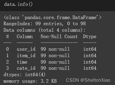
use Amazon-Electronics Generating a new dataset completes the actual operation .

The original data is json Format , We extract the required information for a preprocessing that contains only user_id, item_id, cate_id, time Four characteristic columns CSV file .
Be careful ：examples There are only 100 Row data is convenient for our lightweight learning

about DIN Features required by the model , Divided into three categories

• Dense features ： Also known as numerical characteristics , For example, salary 、 Age , stay DIN We do not use this type of feature .
• Sparse features ： Also known as category type feature , Such as gender 、 Education . In this tutorial Sparse Feature directly LabelEncoder Coding operation , Map the original category string to a number , In the model, we will generate Embedding vector .
• Sequence features ： Sequence characteristics , For example, user history clicks item_id Sequence 、 Historical shop sequence, etc , How to extract sequence features , Are we in DIN A key point in learning , It's also DIN One of the main innovations .

It is important to understand the composition of data sets here . In practice, we try to determine the characteristics of historical sequences from the original data set （ With the help of create_seq_features), The features are as follows ：

Because it corresponds to different types of features , Models can be treated in different ways , So we still need to use rechub The built-in data class of is used for feature type annotation

In this case , Because we use user_id,item_id and item_cate These three categories feature , Use user's item_id and cate As a sequence feature . stay torch-rechub We just need to call DenseFeature, SparseFeature, SequenceFeature These three categories , Each type of feature can be processed automatically and correctly .

Finally, convert the input data into dictionary form

2.4.2 Training

Then define model training

epoch: 0
train: 100%|██████████| 1/1 [00:00<00:00,  6.56it/s]
validation: 100%|██████████| 1/1 [00:00<00:00,  7.16it/s]
epoch: 0 validation: auc: 1.0
epoch: 1
train: 100%|██████████| 1/1 [00:00<00:00,  6.55it/s]
validation: 100%|██████████| 1/1 [00:00<00:00,  7.57it/s]
epoch: 1 validation: auc: 1.0
epoch: 2
train: 100%|██████████| 1/1 [00:00<00:00,  6.40it/s]
validation: 100%|██████████| 1/1 [00:00<00:00,  6.76it/s]
epoch: 2 validation: auc: 1.0
validation: 100%|██████████| 1/1 [00:00<00:00,  6.92it/s]test auc: 1.0

Because of the small amount of data ,3 individual epoch It has achieved good results

Reference material

1. torch-rechub
2. FunRec course
3. Introduction to recommender system