当前位置:网站首页>[Video] visual interpretation of Markov chain principle and Mrs example of R language region conversion | data sharing
[Video] visual interpretation of Markov chain principle and Mrs example of R language region conversion | data sharing
2022-07-25 13:07:00 【51CTO】
Markov chain is from a “ state ”( A situation or set of values ) Jump to another “ state ” The mathematical system of . This paper introduces Markov chain and a simple state transition model , This model constitutes a hidden Markov model (HMM) The special case of . From an application point of view , These models are evaluating the economy / Market status data ( See the end of the article for data acquisition methods ) Very useful . The discussion here focuses on the scientific nature of using these models .
video : Visual interpretation and of Markov chain principle R Language locale conversion Markov regime switching example
Visual interpretation and of Markov chain principle R Language locale conversion Markov regime switching example
, Duration 07:25
for example , If you make a Markov chain model of infant behavior , You may “ play ”、“ having dinner ”、“ sleep ” and “ Cry ” As a state , Together with other behaviors, they can form “ The state space ”: A list of all possible states . Besides , Above the state space , Markov chains tell you to jump from a state or “ transformation ” The probability of reaching any other state —— for example , The baby who is playing is likely to fall asleep in the next state without crying for five minutes .
A simple two-state Markov chain is shown below .

There are two states in our state space (A and B), Yes 4 Possible transformations ( No 2 Kind of , Because the state can be converted back to itself ). If we were “A”, We can transition to “B” Or stay “A”. If we were “B”, We can transition to “A” Or stay “B”. In these two state diagrams , The probability of switching from any state to any other state is 0.5.

Of course , Real modelers do not always draw Markov chain diagrams . contrary , They use “ transition matrix ” To calculate the transition probability . Each state in the state space contains once as rows and columns , And each cell in the matrix tells you the probability of switching from its row state to its column state . therefore , In the matrix , The function of the cell is the same as that of the arrow in the figure .
If you add a state to the state space , We add a row and a column , Add a cell to each existing column and row . This means that when we add states to Markov chains , The number of cells increased twice . therefore , Unless you want to draw a Markov chain diagram of jungle gym , Otherwise, the transformation matrix will come in handy soon .

One use of Markov chains is to include real-world phenomena in computer simulations . for example , We may want to check the overflow frequency of the new dam , It depends on the number of consecutive rainy days . To build this model , We start from the following rainy days (R) And sunny days (S) Start :
One way to simulate this weather is to just say “ It rains half the day . therefore , In our simulation , available everyday 50% The probability of rain .”
This rule will generate the following sequence in the simulation :

Have you noticed that the above sequence looks different from the original ? The second sequence seems to jump around , And the first one ( Real data ) Seems to have “ viscosity ”. In actual data , If one day is sunny (S), Then the next day is more likely to be sunny .
We can use two-state Markov chains to narrow this “ viscosity ”. When Markov chain is in “R” In the state of , It has 0.9 The probability of staying in place , Yes 0.1 The opportunity to leave “S” state . Again ,“S” The state is 0.9 The probability remains the same , And there are 0.1 The opportunity to switch to “R” state .

In meteorologists 、 ecologist 、 Computer scientists 、 Financial engineers and others who need to model big phenomena , Markov chains can become very large and powerful . for example , Google's algorithm for determining the order of search results , be called PageRank, It's a Markov chain .
Markov regime transfer model Markov regime switching
This paper introduces a simple state transition model , This model constitutes a hidden Markov model (HMM) The special case of . These models fit the non stationarity in time series data .
Basic case
HMM The main challenge is to predict the hidden parts . How do we identify “ It's not observable ” Things of ?HMM The idea is to predict the potential from the observable .
Analog data
To demonstrate , We're going to prepare some data and try to reverse guess . Each state has a different mean and volatility .
theta_v <- data.frame(t(c(2.00,-2.00,1.00,2.00,0.95,0.85))) kable(theta_v, "html", booktabs = F,escape = F) %>% kable_styling(position = "center")

As shown in the table above , state s = 2 become “ bad ” state , The process x_t Showing high variability . therefore , Stay in the State 2 It's more likely than staying in the state 1 It's very unlikely that .
Markov process
To simulate the process x\_t , We start by simulating Markov processes s\_t Start . To simulate T During the process , First , We need to build a given p_ {11} and p_ {22} The transformation matrix of . secondly , We need to start from a given state s\_1 = 1 Start . from s\_1 = 1 Start , We know there are 95% The probability of being in a state 1, Yes 5% The probability of entering the State 2.
P <- matrix(c(p11,1-p22,1-p11,p22),2,2) P\[1,\]
## \[1\] 0.95 0.05
Because of its previous state , simulation s_t It's recursive . therefore , We need to construct a loop :
for(t in 2:T_end) { s <- c(s,st(s\[t-1\])) } plot(s, pch = 20,cex = 0.5)

The picture above illustrates the process s_t The durability of . in the majority of cases , state 1 Of “ Realization ” More than state 2. actually , This can be determined by the probability of stability , The stability probability is expressed by the following formula :
P_stat\[1,\]
## \[1\] 0.75 0.25
therefore , Yes 15% The probability of being in 1 state , But there is 25% The probability of being in a state 2. This should be reflected in the simulation process s, thus
mean(s==1)
## \[1\] 0.69
Because we use 100 A small sample of two cycles , So we observe that the probability of stability is 69%, Close but not quite equal to 75%.
result
Given a simulated Markov process , The simulation of the results is very simple . A simple trick is to simulate

Of T Period and T cycle . then , Given s\_t The simulation , We create result variables for each state x\_t .
plot(x~t_index, pch = 20) points(x\[s == 2\]~t_index\[s==2\],col = 2)

Although overall, the time series seems to be stable , But we see some cycles ( Highlighted in red ) Showing high volatility . One might suggest that , There is a structural disruption to the data , Or the regional system has changed , The process x_t Getting bigger and bigger , With more negative values . Even so , It's always easier to explain afterwards . The main challenge is to identify the situation .
Estimated parameters
In this section , I will use R Software manual ( Start from scratch ) And non manual statistical decomposition . In the former , I'll show you how to construct the likelihood function , Then the constrained optimization problem is used to estimate the parameters .
Likelihood function - The numerical part
First , We need to create one to Theta Vector is the main input function . secondly , We need to set up a MLE Optimization problem .
Before optimizing the likelihood function . Let's look at how it works . Suppose we know the parameters Theta Vector , And we're interested in using x_t Evaluate the hidden state of data over time .

obviously , The sum of each filter for both States should be 1. look , We can be in the State 1 Or status 2.
all(round(apply(Filter\[,-1\],1,sum),9) == 1)
## \[1\] TRUE
Because we designed this data , So we know the State 2 A period of .
plot(Filter\[,3\]~t_index, type = "l", ylab = expression(xi\[2\])) points(Filter\[s==2,3\]~t_index\[s==2\],pch = 20, col = 2)

The advantage behind the filter is that it only uses x_t To identify potential states . We observed that , state 2 The main state of the filter is 2 Increase when it happens . This can be proved by increasing the probability of emitting red dots , The red dot indicates the state 2 Time period of occurrence . For all that , There are still some big problems . First , It assumes that we know the parameters Theta , And actually we need to estimate that , And then infer on this basis . secondly , All of these are constructed in the sample . From a practical point of view , Decision makers are interested in the probability of forecasting and its impact on future investments .
Manual estimation
In order to optimize the HMM_Lik function , I will need to perform two additional steps . The first is to establish an initial estimate , As the starting point of the search algorithm . secondly , We need to set constraints to verify that the estimated parameters are consistent , That is, non negative volatility and between 0 and 1 Probability value between .
First step , I use samples to create initial parameter vectors Theta_0
In the second step , I put constraints on the estimates
Please note that , The initial vector of the parameter should satisfy the constraint condition
all(A%*%theta0 >= B)
## \[1\] TRUE
Last , Think about it , By constructing most optimization algorithms, we can search the minimum point . therefore , We need to change the output of the likelihood function to a negative value .
## $par ## \[1\] 1.7119528 -1.9981224 0.8345350 2.2183230 0.9365507 0.8487511 ## ## $value ## \[1\] 174.7445 ## ## $counts ## function gradient ## 1002 NA ## ## $convergence ## \[1\] 0 ## ## $message ## NULL ## ## $outer.iterations ## \[1\] 3 ## ## $barrier.value ## \[1\] 6.538295e-05
For inspection MLE Whether the value is consistent with the real parameter , We plot the relationship between the estimated value and the true value :
plot(opt$par ~ theta_known,pch = 20,cex=2,ylab="MLE",xlab = "True") abline(a=0,b=1,lty=2)
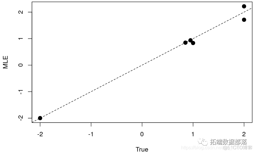
Overall speaking , We observed very consistent estimates .
Estimate
I'll show you how to use r The software reproduces the results of manual estimation .
If we're going to ignore any regime switching in the process , We can simply put the parameters mu and sigma It is estimated that
kable(mod_est, "html", booktabs = F,escape = F) %>% kable_styling(position = "center")

On average, , We should expect the process average to be about 1, namely

. This is derived from the law of expectation , We know that

EX <- 0.75\*2 + 0.25\*-2 EX
## \[1\] 1
For volatility , Apply the same logic .
## \[1\] 2.179449
We noticed that , The consistency of regression estimates and volatility is higher than the mean .
The above view is , The estimates do not cover the true nature of the data . If we assume that the data is stable , So we mistakenly estimate that the average of the process is 62%. however , meanwhile , We know by construction that the process shows two average results - One positive and one negative . So is volatility .
To reveal these patterns , Let's show how to use the above linear model to build the regional transfer model :
The main input is the fitting model , mod We generalize it to fit the transition state . the second k It's the number of districts . Because we know we have to deal with two states , So set it to 2. however , actually , We need to refer to an information standard to determine the optimal number of states . According to the definition , We have two parameters , mean value mu\_s And volatility sigma\_s . therefore , Let's add a true / false Vector to indicate the parameter being transferred . In the above order , We allow both parameters to be transferred . Last , We can specify whether the estimation process is using parallel computing .
To understand the output of the model , Let's take a look
## Markov Switching Model ## ## ## AIC BIC logLik ## 352.2843 366.705 -174.1422 ## ## Coefficients: ## (Intercept)(S) Std(S) ## Model 1 1.711693 0.8346013 ## Model 2 -2.004137 2.2155742 ## ## Transition probabilities: ## Regime 1 Regime 2 ## Regime 1 0.93767719 0.1510052 ## Regime 2 0.06232281 0.8489948
The output above mainly reports the six estimation parameters we tried to estimate manually . First , The coefficient table reports the mean and fluctuation of each state . Model 1 The average value of is 1.71, Volatility is close to 1. Model 2 The average value of is -2, The volatility is about 2. obviously , The model identifies two different states with different means and volatility for the data . secondly , At the bottom of the output , The fitted model reports the transition probability .

Interestingly , In terms of filters in each state , We compare the state retrieved from the package with the state manually extracted . According to the definition , You can use graph functions To understand the smoothing probability and the determined scheme .
par(mar = 2*c(1,1,1,1),mfrow = c(2,1))
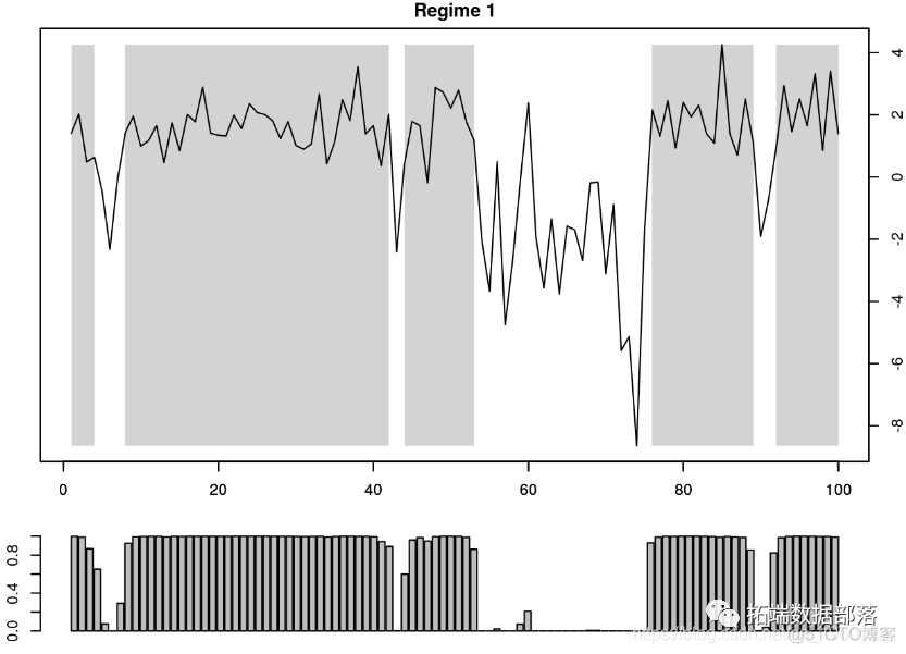
The graph at the top shows the process over time x_t , The gray shaded area indicates

Time period . let me put it another way , The gray area represents the state 1 The dominant period of time .
plot(x~t_index,type ="l",col = 0,xlim=c(1,100))

The filter detects a second state in one cycle . This happens because in this case , The return is the smoothing probability , That is to say, after realizing the whole sample T The probability of being in each state after , namely

. On the other hand , Inferential probabilities from manual estimation .
in any case , Because we know the true value of the State , So we can determine if we are in a real state . We use black dots to highlight the state in the figure above 2. in general , We observe that the model performs very well in detecting the state of the data . The only exception is 60 God , The inference probability is greater than 50%. To see how often the probability of inference is correct , We run the following command
mean(Filter$Regime_1 == (s==1)*1)
## \[1\] 0.96
Conclusion
There are still many challenges in real data implementation . First , We don't have the knowledge of the data generation process . secondly , States don't have to be realized . therefore , These two problems may undermine the reliability of the regime transfer model . In application , Such models are often deployed to assess economic or market conditions . In terms of decision making , This can also provide interesting suggestions for policy allocation .

Excerpts from this article 《R Language Markov regime transfer model Markov regime switching》
边栏推荐
- 如何理解Keras中的指标Metrics
- Want to go whoring in vain, right? Enough for you this time!
- Zero basic learning canoe panel (12) -- progress bar
- 深度学习的训练、预测过程详解【以LeNet模型和CIFAR10数据集为例】
- Detailed explanation of switch link aggregation [Huawei ENSP]
- B tree and b+ tree
- [problem solving] ibatis.binding BindingException: Type interface xxDao is not known to the MapperRegistry.
- 力扣 83双周赛T4 6131.不可能得到的最短骰子序列、303 周赛T4 6127.优质数对的数目
- Simple understanding of flow
- 全球都热炸了,谷歌服务器已经崩掉了
猜你喜欢

【AI4Code】《Contrastive Code Representation Learning》 (EMNLP 2021)

程序的内存布局

AtCoder Beginner Contest 261E // 按位思考 + dp

VIM tip: always show line numbers
![[problem solving] org.apache.ibatis.exceptions PersistenceException: Error building SqlSession. 1-byte word of UTF-8 sequence](/img/fd/245306273e464c04f3292132fbfa2f.png)
[problem solving] org.apache.ibatis.exceptions PersistenceException: Error building SqlSession. 1-byte word of UTF-8 sequence

A turbulent life

Zero basic learning canoe panel (16) -- clock control/panel control/start stop control/tab control

卷积核越大性能越强?一文解读RepLKNet模型

word样式和多级列表设置技巧(二)
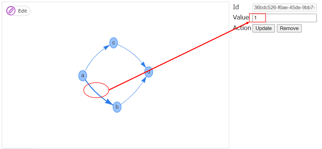
业务可视化-让你的流程图'Run'起来(3.分支选择&跨语言分布式运行节点)
随机推荐
如何理解Keras中的指标Metrics
Lu MENGZHENG's "Fu of broken kiln"
Want to go whoring in vain, right? Enough for you this time!
Shell常用脚本:检测某域名、IP地址是否通
[300 opencv routines] 239. accurate positioning of Harris corner detection (cornersubpix)
conda常用命令:安装,更新,创建,激活,关闭,查看,卸载,删除,清理,重命名,换源,问题
公安部:国际社会普遍认为中国是世界上最安全的国家之一
Mid 2022 review | latest progress of large model technology Lanzhou Technology
web安全入门-UDP测试与防御
clickhouse笔记03-- Grafana 接入ClickHouse
2022.07.24 (lc_6125_equal row and column pairs)
Shell常用脚本:判断远程主机的文件是否存在
Detailed explanation of flex box
业务可视化-让你的流程图'Run'起来(3.分支选择&跨语言分布式运行节点)
Seven lines of code made station B crash for three hours, but "a scheming 0"
Zero basic learning canoe panel (12) -- progress bar
Intval MD5 bypass [wustctf2020] plain
[today in history] July 25: IBM obtained the first patent; Verizon acquires Yahoo; Amazon releases fire phone
深度学习的训练、预测过程详解【以LeNet模型和CIFAR10数据集为例】
【视频】马尔可夫链蒙特卡罗方法MCMC原理与R语言实现|数据分享