Understand 12 convolution methods (including 1x1 convolution, transpose convolution and deep separable convolution)

Click on the above “ Xiaobai studies vision ”, Optional plus " Star standard " or “ Roof placement ”

 Heavy dry goods , First time delivery 

We all know the importance of convolution , But you know what convolution is in the field of deep learning , How many kinds are there ？ Researchers Kunlun Bai Recently released a convolution article on deep learning , This paper introduces various convolutions and their advantages in the field of deep learning in a simple and understandable way . Since the original text is too long , The heart of the machine selects some of the contents to introduce ,2、4、5、9、11、12 Please refer to the original text .

If you've heard of different kinds of convolution in deep learning （ such as 2D / 3D / 1x1 / Transposition / expansion （Atrous）/ Space can be divided / Depth can be divided into / Flattening / grouping / Mix wash group convolution ）, And I don't know what they mean , So this article is for you , Can help you understand how they actually work .

In this article , I will summarize several convolutions commonly used in deep learning , And try to explain them in a way that everyone can understand . In addition to this article , There are also some good articles on this topic , Please refer to the original text .

I hope this article can help you build an intuitive understanding of convolution , And become a useful reference for your research or study .

Contents of this article

1. Convolution and cross correlation

2. Convolution in deep learning （ Single channel version , Multi channel version ）

3. 3D Convolution

4. 1×1 Convolution

5. Convolution arithmetic

6. Transposition convolution （ Deconvolution 、 Chessboard effect ）

7. Expansion convolution

8. Separable convolution （ Spatially separable convolution , Deep separable convolution ）

9. Flat convolution

10. Grouping convolution

11. Mix wash group convolution

12. Point by point group convolution

One 、 Convolution and cross correlation

In signal processing 、 Image processing and other engineering / In the field of Science , Convolution is a widely used technique . In the field of deep learning , Convolutional neural networks （CNN） This model architecture is named after this technology . however , Convolution in the field of deep learning is essentially a signal / Cross correlation in the field of image processing （cross-correlation）. There are subtle differences between the two operations .

Don't go into too much detail , We can see the difference . On the signal / The field of image processing , Convolution is defined as ：

Its definition is the integral of the product obtained by multiplying one of the two functions after inversion and displacement . The following visualization shows this idea ：

Convolution in signal processing . filter g After reversing , Then slide along the horizontal axis . In every position , We all calculate f And after reversal g The area of the intersection area between . The area of this intersecting region is the convolution value at a specific location .

here , function g It's the filter . It is reversed and then slides along the horizontal axis . In every position , We all calculate f And after reversal g The area of the intersection area between . The area of this intersecting region is the convolution value at a specific location .

On the other hand , Cross correlation is the sliding dot product or sliding inner product between two functions . The filters in the correlation are not reversed , Instead, it slides directly over the function f.f And g The cross region between them is cross-correlation . The following figure shows the difference between convolution and cross-correlation .

The difference between convolution and cross-correlation in signal processing

In deep learning , The filter in convolution is not inverted . Strictly speaking , This is cross-correlation . We essentially perform element by element multiplication and addition . But in deep learning , It is more convenient to call it convolution directly . It's no problem , Because the weight of the filter is learned in the training stage . If the inversion function in the above example g It's the right function , So after training , The learned filter will look like an inverted function g. therefore , Before training , There is no need to reverse the filter first, as in a real convolution .

Two 、3D Convolution

In the explanation of the previous section , We see that we are actually talking about a 3D Volume performs convolution . But generally speaking , We still call it... In deep learning 2D Convolution . This is 3D On volume data 2D Convolution . The filter depth is the same as the input layer depth . This 3D The filter moves only in two directions （ The height and width of the image ）. The output of this operation is a 2D Images （ There is only one channel ）.

Naturally, ,3D Convolution does exist . This is a 2D Generalization of convolution . The following is 3D Convolution , The filter depth is less than the input layer depth （ Nuclear size < Channel size ）. therefore ,3D The filter can be in all three directions （ The height of the image 、 Width 、 passageway ） Move up . In every position , Element by element multiplication and addition will provide a value . Because the filter is slipping over a 3D Space , So the output value is also pressed 3D Spatial arrangement . In other words, the output is a 3D data .

stay 3D The convolution ,3D The filter can be in all three directions （ The height of the image 、 Width 、 passageway ） Move up . In every position , Element by element multiplication and addition will provide a value . Because the filter is slipping over a 3D Space , So the output value is also pressed 3D Spatial arrangement . In other words, the output is a 3D data .

And 2D Convolution （ It's encoded 2D The spatial relationship of the targets in the domain ） similar ,3D Convolution can describe 3D The spatial relationship of objects in space . For some applications （ For example, in biomedical imaging 3D Division / restructure ） for , In this way 3D Relationships are important , For example CT and MRI in , Targets like blood vessels will be in 3D There are twists and turns in the space .

3、 ... and 、 Transposition convolution （ Deconvolution ）

For many applications of many network architectures , We often need to convert in the opposite direction to the normal convolution , That is, we want to perform up sampling . Examples include generating high-resolution images and mapping low dimensional feature maps to high-dimensional space , For example, in automatic encoder or shape and meaning segmentation .（ In the latter case , Shape and meaning segmentation will first extract the feature map in the encoder , Then restore the original image size in the decoder , Make it possible to classify each pixel in the original image .）

The traditional way to implement up sampling is to apply interpolation scheme or create rules manually . However, modern architectures such as neural networks tend to let the network learn the appropriate transformation automatically , No human intervention required . To do this , We can use transpose convolution .

Transposed convolution is also called deconvolution or fractionally strided convolution. however , Need to point out that 「 Deconvolution （deconvolution）」 It's not the right name , Because transpose convolution is not a signal / The real deconvolution defined in the field of image processing . Technically speaking , Deconvolution in signal processing is the inverse of convolution . But this is not the operation . therefore , Some authors strongly object to calling transposed convolution deconvolution . It is called deconvolution mainly because it is simple to say so . Later we will explain why it is more natural and appropriate to call this operation transpose convolution .

We can always use direct convolution to realize transpose convolution . For the example below , We're in a 2×2 The input of （ Surrounded by 2×2 Zero padding per unit step ） Apply a 3×3 Transpose convolution of kernels . The size of the upsampling output is 4×4.

take 2×2 The input of is sampled into 4×4 Output

Interestingly , By applying various fills and steps , We can put the same 2×2 The input image is mapped to different image sizes . below , Transpose convolution is used on the same sheet 2×2 Input on （ A zero is inserted between the inputs , And added around 2×2 Zero padding per unit step ）, The size of the resulting output is 5×5.

take 2×2 The input of is sampled into 5×5 Output

Observing the transposed convolution in the above example can help us build some intuitive understanding . But in order to generalize its application , It is useful to know how it can be realized by matrix multiplication of the computer . From this point we can also see why 「 Transposition convolution 」 Is the right name .

In convolution , We define C Is the convolution kernel ,Large Input image for ,Small Output image for . After a convolution （ Matrix multiplication ） after , We downsample large images into small images . The convolution of this matrix multiplication is implemented in accordance with ：C x Large = Small.

The following example shows how this operation works . It flattens the input to 16×1 Matrix , The convolution kernel is transformed into a sparse matrix （4×16）. then , Use matrix multiplication between sparse matrix and flattened input . after , And then the resulting matrix （4×1） Convert to 2×2 Output .

Matrix multiplication of convolution ： take Large The input image （4×4） Convert to Small Output image （2×2）

Now? , If we multiply the transpose of the matrix on both sides of the equation CT, With the help of 「 The multiplication of a matrix and its transposed matrix yields an identity matrix 」 This is the nature of , So we can get the formula CT x Small = Large, As shown in the figure below .

Matrix multiplication of convolution ： take Small The input image （2×2） Convert to Large Output image （4×4）

Here you can see , We performed upsampling from small images to large images . This is exactly what we want to achieve . Now? . You will know 「 Transposition convolution 」 The origin of the name .

For the arithmetic explanation of transpose matrix, please refer to ：https://arxiv.org/abs/1603.07285 

Four 、 Expansion convolution （Atrous Convolution ）

Extended convolution is introduced by these two papers ：

• https://arxiv.org/abs/1412.7062;

• https://arxiv.org/abs/1511.07122

This is a standard discrete convolution ：

The expansion convolution is as follows ：

When l=1 when , The expanded convolution becomes the same as the standard convolution .

Expansion convolution

Intuitively , Expanding convolution is to make the kernel by inserting spaces between the kernel elements 「 inflation 」. New parameters l（ Expansion rate ） Indicates the extent to which we wish to widen the nuclear . The implementation may vary , But it's usually between the nuclear elements l-1 A space . The following shows l = 1, 2, 4 Nuclear size at .

Expand the receptive field of convolution . We basically do not need to add additional costs to have a larger receptive field .

In this image ,3×3 The red dot of indicates that after convolution , The output image is 3×3 Pixels . Although the outputs of all three extended convolutions are of the same size , But the receptive field observed by the model is very different .l=1 When feeling wild for 3×3,l=2 When is 7×7.l=3 when , The size of the receptive field increases to 15×15. Interestingly , The number of parameters associated with these operations is equal . We 「 Observe 」 There is no extra cost for a larger receptive field . therefore , The extended convolution can be used to increase the receptive field of the output unit cheaply , Without increasing its core size , This is especially effective when multiple extended convolutions are stacked on top of each other .

The paper 《Multi-scale context aggregation by dilated convolutions》 The authors of this paper construct a network with multiple extended convolution layers , And the expansion rate l Each layer increases exponentially . thus , The size of effective receptive field increases exponentially with the layer , The number of parameters only increases linearly .

In this paper, the function of extended convolution is to systematically aggregate multiple proportions of context information , Without losing resolution . This paper shows that the proposed module can improve the performance of the system at that time （2016 year ） The accuracy of the current best shape and meaning segmentation system . Please refer to that paper for more information .

5、 ... and 、 Separable convolution

Some neural network architectures use separable convolution , such as  MobileNets. Separable convolution includes space separable convolution and depth separable convolution .

1、 Spatially separable convolution

Spatially separable convolution is the operation of the image 2D Spatial dimension , I.e. height and width . Conceptually , Spatially separable convolution is the decomposition of a convolution into two separate operations . For the following example ,3×3 Of Sobel The nucleus is divided into one 3×1 Nuclear and a 1×3 nucleus .

Sobel The approval can be divided into one 3x1 And a 1x3 nucleus

In convolution ,3×3 The kernel convolutes directly with the image . In space separable volume product ,3×1 The kernel is first convoluted with the image , And then apply 1×3 nucleus . such , To do the same, just 6 Parameters , instead of 9 individual .

Besides , Using spatially separable convolution requires less matrix multiplication . Give me a concrete example ,5×5 Image and 3×3 Convolution of kernels （ Stride =1, fill =0） Ask for in 3 Scan the nucleus horizontally at three positions （ also 3 A vertical position ）. All in all 9 A place , Represented by the points in the following figure . In every position , Will be applied 9 Times element by element multiplication . All in all 9×9=81 Times multiplication .

have 1 Standard convolution of channels

On the other hand , For spatially separable convolution , We started with 5×5 Apply a... To the image of 3×1 Filter . We can be at the level 5 Positions and verticals 3 Scan such a nucleus at three locations . All in all 5×3=15 A place , Represented by the points in the following figure . In every position , Will be applied 3 Times element by element multiplication . All in all 15×3=45 Times multiplication . Now we have a 3×5 Matrix . This matrix is connected with a 1×3 Kernel convolution , That is, at the level 3 Positions and verticals 3 Scan this matrix at positions . For this 9 Each of the positions , application 3 Times element by element multiplication . This step requires 9×3=27 Times multiplication . therefore , Overall speaking , Spatially separable convolution requires 45+27=72 Times multiplication , Less than normal convolution .

have 1 Spatially separable convolution of channels

Let's generalize the above example . Suppose we now apply convolution to a sheet N×N On the image of , Convolution kernels for m×m, The stride is 1, Fill in with 0. Traditional convolution requires (N-2) x (N-2) x m x m Times multiplication , Spatially separable convolution requires N x (N-2) x m + (N-2) x (N-2) x m = (2N-2) x (N-2) x m Times multiplication . The computational cost ratio of spatially separable convolution and standard convolution is ：

Because the image size N Much larger than the filter size （N>>m）, So this ratio becomes 2/m. in other words , In this progressive situation （N>>m） Next , When the filter size is 3×3 when , The computational cost of spatially separable convolution is that of standard convolution 2/3. The filter size is 5×5 This value is 2/5; The filter size is 7×7 Otherwise 2/7.

Although space can be divided into volumes to save costs , But deep learning rarely uses it . One of the main reasons is that not all nuclei can be divided into two smaller nuclei . If we replace all traditional convolutions with spatially separable convolutions , Then we limit ourselves to searching all possible cores during the training process . The training result may be suboptimal .

2、 Deep separable convolution

Now let's look at the depth separable convolution , This is much more common in the field of deep learning （ such as MobileNet and Xception）. Deep separable convolution consists of two steps ： Deep convolution kernel 1×1 Convolution .

Before describing these steps , It is necessary to review what we introduced before 2D Convolution kernel 1×1 Convolution . First, quickly review the standard 2D Convolution . Take a concrete example , Suppose the size of the input layer is 7×7×3（ high × wide × passageway ）, The size of the filter is 3×3×3. Pass through with a filter 2D After convolution , The size of the output layer is 5×5×1（ There is only one channel ）.

Used to create only 1 The output standard of the layer 2D Convolution , Use 1 A filter

Generally speaking , Multiple filters are applied between the two neural network layers . Suppose we have 128 A filter . In the application of this 128 individual 2D After convolution , We have 128 individual 5×5×1 Output map of （map）. Then we stack these maps into a size of 5×5×128 A single layer . Through this operation , We can put the input layer （7×7×3） To the output layer （5×5×128）. Spatial dimension （ That is, height and width ） It's going to get smaller , And the depth will increase .

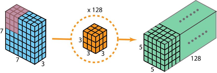
Used to create a 128 The output standard of the layer 2D Convolution , To use 128 A filter  

Now use the depth separable convolution , See how we can implement the same transformation .

First , We apply depth convolution to the input layer . But we don't use 2D The size in convolution is 3×3×3 A single filter , They are used separately 3 A nuclear . The size of each filter is 3×3×1. Each kernel is convoluted with a channel of the input layer （ Only one channel , Not all channels ！）. Each such convolution can provide a value of 5×5×1 The map of . Then we stack these maps together , Create a 5×5×3 Image . After this operation , We get a size of 5×5×3 Output . Now we can reduce the spatial dimension , But the depth is the same as before .

Deep separable convolution —— First step ： We don't use 2D The size in convolution is 3×3×3 A single filter , They are used separately 3 A nuclear . The size of each filter is 3×3×1. Each kernel is convoluted with a channel of the input layer （ Only one channel , Not all channels ！）. Each such convolution can provide a value of 5×5×1 The map of . Then we stack these maps together , Create a 5×5×3 Image . After this operation , We get a size of 5×5×3 Output .

In the second step of deep separable convolution , To expand the depth , We apply a core size of 1×1×3 Of 1×1 Convolution . take 5×5×3 Input image with each 1×1×3 Kernel convolution of , The obtained size is 5×5×1 The map of .

therefore , In the application of 128 individual 1×1 After convolution , We get a size of 5×5×128 The layer .

Deep separable convolution —— The second step ： Apply multiple 1×1 Convolution to modify the depth .

Through these two steps , The depth separable convolution will also transform the input layer （7×7×3） Transform to output layer （5×5×128）.

The following figure shows the whole process of deep separable convolution .

The whole process of deep separable convolution

therefore , What are the advantages of deep separable convolution ？ efficiency ！ Compared with 2D Convolution , Deep separable convolution requires much less operation .

Recall our 2D The computational cost of convolution example . Yes 128 individual 3×3×3 A core has moved 5×5 Time , That is to say 128 x 3 x 3 x 3 x 5 x 5 = 86400 Times multiplication .

What about separable convolution ？ In the first depth convolution step , Yes 3 individual 3×3×1 Nuclear movement 5×5 Time , That is to say 3x3x3x1x5x5 = 675 Times multiplication . stay 1×1 The second step of convolution , Yes 128 individual 1×1×3 Nuclear movement 5×5 Time , namely 128 x 1 x 1 x 3 x 5 x 5 = 9600 Times multiplication . therefore , Depth separable convolution is common 675 + 9600 = 10275 Times multiplication . The cost is probably only 2D Convolution 12%！

therefore , For images of any size , If we apply depth separable convolution , How much time can we save ？ Let's generalize the above example . Now? , For size H×W×D The input image of , If you use Nc Size is h×h×D Nuclear implementation of 2D Convolution （ The stride is 1, Fill in with 0, among h It's even ）. To put the input layer （H×W×D） Transform to output layer （(H-h+1)x (W-h+1) x Nc）, The total number of multiplications required is ：

Nc x h x h x D x (H-h+1) x (W-h+1)

On the other hand , For the same transformation , The number of multiplications required for deep separable convolution is ：

D x h x h x 1 x (H-h+1) x (W-h+1) + Nc x 1 x 1 x D x (H-h+1) x (W-h+1) = (h x h + Nc) x D x (H-h+1) x (W-h+1)

Then the depth can be divided into convolution and 2D The multiplication ratio required for convolution is ：

The output layer of most modern architectures usually has many channels , It can reach hundreds or even thousands . For such a layer （Nc >> h）, Then the above formula can be reduced to 1 / h². Based on this , If you use 3×3 filter , be 2D The number of multiplications required for convolution is deeply separable convolution 9 times . If you use 5×5 filter , be 2D The number of multiplications required for convolution is deeply separable convolution 25 times .

Is there any harm in using deep separable convolution ？ Of course there are . Deep separable convolution reduces the number of parameters in convolution . therefore , For smaller models , If we use depth separable convolution instead of 2D Convolution , The ability of the model may decline significantly . therefore , The resulting model may be suboptimal . however , If used properly , Deep separable convolution can help you achieve efficiency improvement without reducing the performance of your model .

6、 ... and 、 Grouping convolution

AlexNet The paper （https://papers.nips.cc/paper/4824-imagenet-classification-with-deep-convolutional-neural-networks.pdf） stay 2012 Grouping convolution was introduced in . The main reason to realize packet convolution is to make network training available in 2 Memory is limited （ Every GPU Yes 1.5 GB Memory ） Of GPU on . Below AlexNet It shows that there are two separate convolution paths in most layers . This is in two GPU Perform model parallelization on （ Of course, if you can use more GPU, How much more GPU Parallelization ）.

The picture is from AlexNet The paper

Here we introduce the working mode of block convolution . First , Typical 2D The steps of convolution are shown in the figure below . In this case , By applying the 128 Size is 3×3×3 The filter of will input layer （7×7×3） Transform to output layer （5×5×128）. In terms of promotion , That is, by applying Dout Size is h x w x Din The core of will be input to the layer （Hin x Win x Din） Transform to output layer （Hout x Wout x Dout）.

The standard 2D Convolution

In group convolution , Filters are divided into different groups . Each group is responsible for a typical 2D Convolution . The following example will help you understand .

Packet convolution with two filter packets

The figure above shows the packet convolution with two filter packets . In each filter group , The depth of each filter is only nominally 2D Half of convolution . Their depth is Din/2. Each filter group contains Dout/2 A filter . The first filter group （ Red ） With the first half of the input layer （[:, :, 0:Din/2]） Convolution , The second filter group （ Orange ） And the second half of the input layer （[:, :, Din/2:Din]） Convolution . therefore , Each filter group creates Dout/2 Channels . As a whole , The two groups create 2×Dout/2 = Dout Channels . Then we stack these channels together , Get to have Dout The output layer of two channels .

1、 Block convolution and depth convolution

You may notice that there are some connections and differences between the block convolution and the depth convolution used in the depth separable convolution . If the number of filter groups is the same as the number of input layer channels , Then the depth of each filter is Din/Din=1. Such filter depth is the same as that in depth convolution .

On the other hand , Now each filter group contains Dout/Din A filter . As a whole , The depth of the output layer is Dout. This is different from the case of depth convolution —— Depth convolution does not change the depth of the layer . In deep separable convolution , The depth of the layer then passes through 1×1 Convolution is extended .

Block convolution has several advantages .

The first advantage is efficient training . Because convolution is divided into multiple paths , Each path can be represented by a different GPU Separate the , So the model can be used in multiple GPU Training on . Compared to a single GPU Complete all tasks on , This is the case in many GPU The parallelization of the model on allows the network to process more images at each step . It is generally believed that model parallelization is better than data parallelization . The latter is to divide the data set into multiple batches , Then train each batch separately . however , When the batch size becomes too small , We are essentially performing random gradient descent , Instead of batch gradient descent . This will result in slower , Sometimes even worse convergence results .

When training very deep neural networks , Grouping convolution will be very important , As in ResNeXt In the .

The picture is from ResNeXt The paper ,https://arxiv.org/abs/1611.05431

The second advantage is that the model will be more efficient , That is, the model parameters will decrease as the number of filter groups increases . In the previous example , Complete standards 2D Convolution has h x w x Din x Dout Parameters . have 2 The packet convolution of filter packets has (h x w x Din/2 x Dout/2) x 2 Parameters . The number of parameters has been halved .

The third advantage is somewhat surprising . Packet convolution may provide more complete than standard 2D Better model for convolution . Another excellent blog has explained this ：https://blog.yani.io/filter-group-tutorial. Here is a brief summary .

The reason is related to the relationship between sparse filters . The following figure shows the correlation of adjacent layer filters . The relationship is sparse .

stay CIFAR10 One of the last training Network-in-Network The correlation matrix of filters in adjacent layers in the model . Highly correlated filter pairs are brighter , The filter with lower correlation is darker . The picture is from ：https://blog.yani.io/filter-group-tutorial

How about the correlation map of the grouping matrix ？

stay CIFAR10 One of the last training Network-in-Network The filter correlation of adjacent layers in the model , The moving pictures respectively show that there are 1、2、4、8、16 Filter groups . The picture is from https://blog.yani.io/filter-group-tutorial

The picture above is for 1、2、4、8、16 When training the model with a filter group , Correlation between filters of adjacent layers . The article put forward a reasoning ：「 The effect of filter grouping is to learn the sparsity of block diagonal structure in the channel dimension …… In the network , Filters with high relevance are learned in a more structured way using filter grouping . In terms of effect , Filter relationships that do not have to be learned are no longer parameterized . This significantly reduces the number of parameters in the network and makes it not easy to over fit , therefore , A regularization like effect enables the optimizer to learn more accurate and efficient deep networks .」

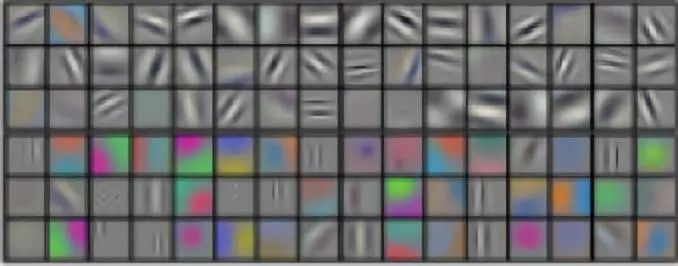
AlexNet conv1 Filter decomposition ： As the author points out , Filter grouping seems to structurally organize the learned filters into two different groups . This picture is from AlexNet The paper .

Besides , Each filter group learns a unique representation of the data . just as AlexNet As the author pointed out , Filter grouping seems to structurally organize the learned filters into two different groups —— Black and white filters and color filters .

In your opinion, there are still some notable points in the convolution of deep learning ？

The good news ！

Xiaobai learns visual knowledge about the planet

Open to the outside world

 download 1：OpenCV-Contrib Chinese version of extension module 

 stay 「 Xiaobai studies vision 」 Official account back office reply ： Extension module Chinese course , You can download the first copy of the whole network OpenCV Extension module tutorial Chinese version , Cover expansion module installation 、SFM Algorithm 、 Stereo vision 、 Target tracking 、 Biological vision 、 Super resolution processing and other more than 20 chapters .


 download 2：Python Visual combat project 52 speak 
 stay 「 Xiaobai studies vision 」 Official account back office reply ：Python Visual combat project , You can download, including image segmentation 、 Mask detection 、 Lane line detection 、 Vehicle count 、 Add Eyeliner 、 License plate recognition 、 Character recognition 、 Emotional tests 、 Text content extraction 、 Face recognition, etc 31 A visual combat project , Help fast school computer vision .


 download 3：OpenCV Actual project 20 speak 
 stay 「 Xiaobai studies vision 」 Official account back office reply ：OpenCV Actual project 20 speak , You can download the 20 Based on OpenCV Realization 20 A real project , Realization OpenCV Learn advanced .


 Communication group 

 Welcome to join the official account reader group to communicate with your colleagues , There are SLAM、 3 d visual 、 sensor 、 Autopilot 、 Computational photography 、 testing 、 Division 、 distinguish 、 Medical imaging 、GAN、 Wechat groups such as algorithm competition （ It will be subdivided gradually in the future ）, Please scan the following micro signal clustering , remarks ：” nickname + School / company + Research direction “, for example ：” Zhang San  +  Shanghai Jiaotong University  +  Vision SLAM“. Please note... According to the format , Otherwise, it will not pass . After successful addition, they will be invited to relevant wechat groups according to the research direction . Please do not send ads in the group , Or you'll be invited out , Thanks for your understanding ~