当前位置:网站首页>Li Hongyi machine learning (2021 Edition)_ P7-9: training skills
Li Hongyi machine learning (2021 Edition)_ P7-9: training skills
2022-07-27 01:13:00 【Although Beihai is on credit, Fuyao can take it】
Catalog
- Related information
- 1、optimize( Adaptive learning rate )
- 2、 classification
- 3、 Batch normalization (Bath Normalization)

Related information
Video link :https://www.bilibili.com/video/BV1JA411c7VT
Original video link :https://speech.ee.ntu.edu.tw/~hylee/ml/2021-spring.html
Leeml-notes Open source project :https://github.com/datawhalechina/leeml-notes
1、optimize( Adaptive learning rate )

In training , A lot of times ,Loss No longer lower , But at this time , In fact, the gradient did not fall to a relatively low level .
One reason is that , The optimized parameters fluctuate at both ends of the gradient Valley , Stagnate :
1.1、 The gradient change rate in different directions is different ( Convex function )
1.1.1、 Applicable scenarios

The loss function is convex, The following figure w and b Express loss Two parameters of , It can be seen that ,b The direction gradient changes slowly ,w The direction gradient changes rapidly .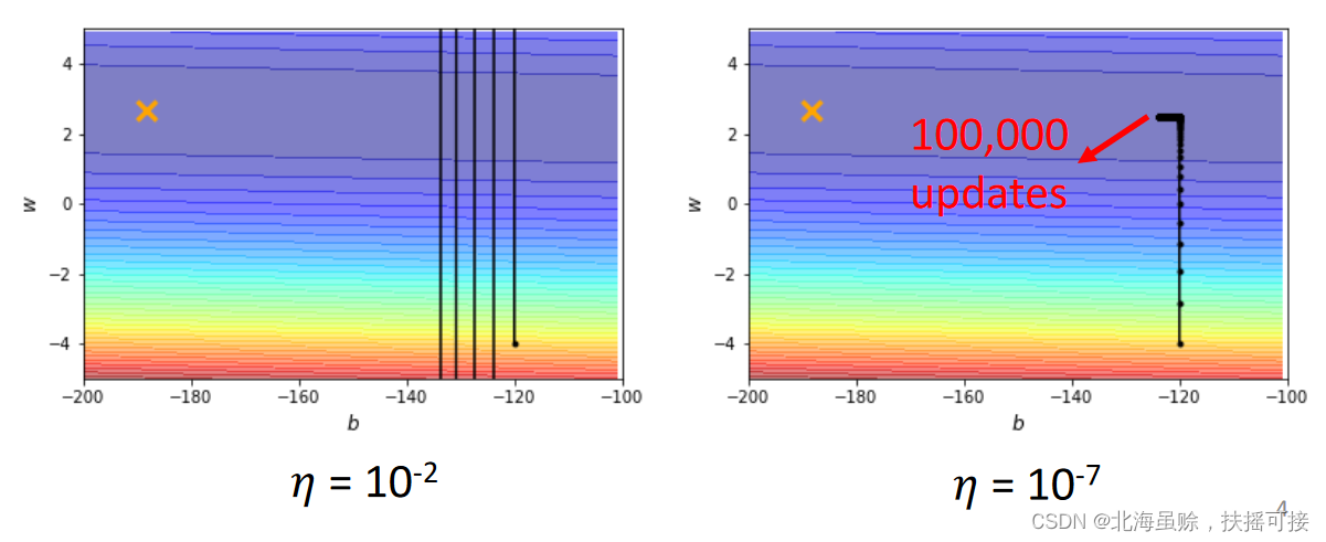
Use the same learning rate , It is difficult to get good results in two dimensions when optimizing , So different parameters need different learning rates .
1.1.2、 Adjust the proportion of learning rate
Original parameter iteration method :
θ i t + 1 = θ i t − η g i t \theta_{i}^{t+1}= \theta _{i}^{t}- {\eta}g_{i}^{t} θit+1=θit−ηgit
Adopt the learning rate adjustment method :
θ i t + 1 = θ i t − η σ i t g i t \theta_{i}^{t+1}= \theta _{i}^{t}- \frac{\eta}{\sigma _{i}^{t}}g_{i}^{t} θit+1=θit−σitηgit
Introduce parameters σ i t \sigma _{i}^{t} σit Adjust the learning rate , There are three calculation methods :
1.1.3、Root Mean Square( Root mean square )
σ i t = 1 t + 1 ∑ i = 0 t ( g i t ) 2 \sigma ^ { t } _ { i } = \sqrt { \frac {1} { t +1 } \sum _ { i = 0 } ^ { t} ( g _ { i } ^{t}) ^ { 2 } } σit=t+11i=0∑t(git)2
The root mean square algorithm takes into account all the values of the gradient calculated by the former , Root mean square . Make the calculation of learning rate in this step , Considering the gradient change of the former , Make this step gradient learn the previous change trend .
Adagrad The algorithm adopts this calculation method .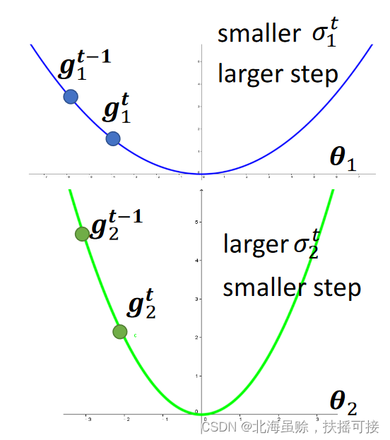
use RMS The optimization effect :
Where the gradient changes greatly , The learning rate changes little , Gradually move ; Dimensions with small gradient changes , The learning rate changes rapidly , There will be a shock , Gradually approaching the best .
1.2、 The gradient in the same direction changes greatly

1.2.1、RMSProp Method
For some other loss, Nonconvex function type , The gradient changes little in a range , But in another range, the gradient changes greatly ; use RMS Method , The learning rate changes slowly , Adopt new methods , Improve the learning rate and change rate . among 0<𝛼<1
σ i t = α ( σ i t − 1 ) 2 + ( 1 − α ) ( g i t ) 2 \sigma_{i}^{t}= \sqrt{\alpha(\sigma _{i}^{t-1})^{2}+(1- \alpha)(g_{i}^{t})^{2}} σit=α(σit−1)2+(1−α)(git)2
RMSProp In the method , For learning rate , The recent gradient has greater influence , The gradient in the past has little effect .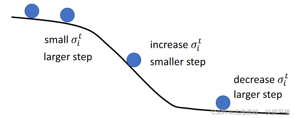
1.2.2、Adam: RMSProp + Momentum

1.3、 Directly adjust the learning rate
In addition to adjusting the proportion of learning rate σ i t \sigma_i^t σit, You can also directly modify the learning rate η t \eta^t ηt, For different times ( Training epoch), Directly modify the learning rate ( Equivalent to macro-control )
θ i t + 1 = θ i t − η t σ i t g i t \theta_{i}^{t+1}= \theta _{i}^{t}- \frac{\eta^t}{\sigma _{i}^{t}}g_{i}^{t} θit+1=θit−σitηtgit
- Learning Rate Decay( Learning rate decline )
 With training , Closer to the destination , So gradually reduce the learning rate .
 - Warm Up( Cosine annealing )

Learning first increases and then decreases ;
In the first place , Calculation statistics σ i t \sigma _{i}^{t} σit With large variance , That is, the statistics are unstable , At this time, the learning rate is relatively high , In the exploratory stage ; When after a while , Learning is relatively stable , The learning rate is lower .
1.4、 summary

θ i t + 1 = θ i t − η t σ i t m i t \theta_{i}^{t+1}= \theta _{i}^{t}- \frac{\eta ^{t}}{\sigma _{i}^{t}}m_{i}^{t} θit+1=θit−σitηtmit
Adjust the learning rate in three ways ( Macroscopic ):
- adjustment σ i t \sigma _{i}^{t} σit: Adjust parameter dependencies , Consider the past learning rate , The vector η \eta η Fine tuning ;
- adjustment η \eta η: Directly adjust the learning rate η t \eta^t ηt, According to training experience , Direct macro-control of learning rate ;
- adjustment m i t m_{i}^{t} mit: Quote momentum m i t m_{i}^{t} mit, Consider the impact of past learning rates , Including direction and value , Help jump out local
minima.
2、 classification
2.1、 Definition
Classification is a method for input data , Output a type of result in a given type ;
2.2、 Network structure

For classified networks , For the same set of data , Perform multiple calculations , Get the same number of outputs as the number of categories , Compare the output results , Finally confirm the classification results .
Different from the regression algorithm , The classification algorithm needs to output results y y y Conduct Softmax Handle , Get the activation value y ′ y^\prime y′.
use Softmax Algorithm , Data can be mapped to 0-1.
2.3、 Loss function
The total loss function of the model is the average of each single data loss function , Loss function calculation includes mean square error and cross entropy function .
- Mean square error Mean Square Error (MSE)

e = ∑ i ( y ^ i − y i ′ ) 2 e= \sum _{i}(\widehat{y}_{i}-y_{i}^{\prime})^{2} e=i∑(yi−yi′)2 - Cross entropy loss function Cross-entropy
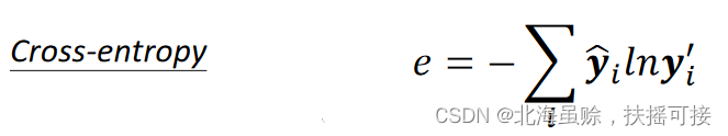
e = − ∑ i y ^ i ln y i ′ e=- \sum _{i}\widehat{y}_{i}\ln y_{i}^{\prime} e=−i∑yilnyi′
The above two loss functions ,Cross-entropy More suitable for classification algorithm . The following is an example , For a three classification algorithm :
The mean square error and cross entropy are used to calculate the loss , The loss calculation diagram is as follows :
The mean square error loss graph is too flat in many places , It's hard to train ;
The loss of cross entropy loss function fluctuates , Easy to train ;
Changing the loss function can change the difficulty of optimization ,( Use Shenluo Tianzheng to flatten the rugged loss function ).
3、 Batch normalization (Bath Normalization)
3.1、 Concept
A function has multiple input characteristics , And the distribution range of the input characteristic data is very different , It is recommended to scale their range , Make the range of different inputs the same . y = b + w 1 x 1 + w 2 x 2 y=b+w_{1}x_{1}+w_{2}x_{2} y=b+w1x1+w2x2
3.2、 reason
x 1 x_1 x1 Yes y The impact of the change is relatively small , therefore w 1 w_1 w1 The influence on the loss function is relatively small , w 1 w_1 w1 There is a small differential for the loss function , therefore w 1 w_1 w1 It is relatively smooth in the direction , Empathy w 2 w_2 w2 The direction is steep .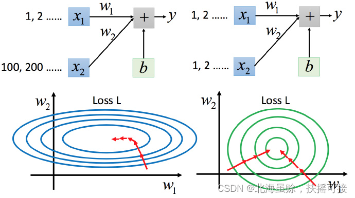
For the case on the left , As mentioned above, there is no need to Adagrad It is difficult to deal with .
- Different learning rates are required in both directions , The learning rate of the same group will not determine it . In the case on the right, it will be easier to update parameters .
- The gradient descent on the left is not towards the lowest point , But along the normal direction of the contour tangent . But green can be towards the center ( The lowest point ) go , It is also more efficient to update parameters .
3.3、 Zoom method
Use the batch normalization method to scale , Zoom to the standard normal distribution .
Each column above is an example , There is a set of characteristics in it .
For each dimension i( Green box ) Calculate the average , Remember to do m i m_i mi; Also calculate the standard deviation , Remember to do σ i \sigma _i σi.
Then use the r( features ) The... In the first example i( data ) Inputs , Subtract the average m i m_i mi, Then divide by the standard deviation σ i \sigma _i σi, The result is that all dimensions are 0, All variances are 1.( Standard normal distribution )
stay DL in , commonly BN It can be used before and after activating the function , When the activation function used is sigmoid when , Generally, it is carried out before the activation function BN.
Conduct BN After the operation , Because sharing μ \mu μ and σ \sigma σ, So all normalization parameters are interrelated .
Sometimes in order to adjust the average , Would be right BN The processed data is processed linearly :
z ~ i = z i − μ σ \tilde{z}^{i}= \frac{z^{i}- \mu}{\sigma} z~i=σzi−μ
z ^ i = γ ⋅ z ~ i + β \widehat{z}^{i}= \gamma \cdot \tilde{z}^{i}+ \beta zi=γ⋅z~i+β
stay test in , Unable to gather enough bath When testing data , Some data values in the training network can be used .

3.4、 Training results

Use BN Can speed up training , And for some difficult training models , You can also finish training .
边栏推荐
- In depth learning report (3)
- The basic concept of how Tencent cloud mlvb technology can highlight the siege in mobile live broadcasting services
- MySQL split table DDL operation (stored procedure)
- 3. 拳王阿里
- SQL learning (3) -- complex query and function operation of tables
- Website log collection and analysis process
- Applet live broadcast, online live broadcast, live broadcast reward: Tencent cloud mobile live broadcast component mlvb multi scene live broadcast expansion
- Game project export AAB package upload Google tips more than 150m solution
- 李宏毅机器学习(2017版)_P5:误差
- Flink 1.15 implements SQL script to recover data from savepointh
猜你喜欢

Naive Bayes Multiclass训练模型

Cannot find a valid baseurl for repo: HDP-3.1-repo-1

Small programs related to a large number of digital collections off the shelves of wechat: is NFT products the future or a trap?

Tencent upgrades the live broadcast function of video Number applet. Tencent's foundation for continuous promotion of live broadcast is this technology called visual cube (mlvb)

FaceNet

李宏毅机器学习(2017版)_P1-2:机器学习介绍

腾讯云直播插件MLVB如何借助这些优势成为主播直播推拉流的神助攻?

下一代互联网:视联网

快来:鼓励高校毕业生返乡创业就业,助力乡村振兴

被围绕的区域
随机推荐
Flink1.11 write MySQL test cases in jdcb mode
Tencent upgrades the live broadcast function of video Number applet. Tencent's foundation for continuous promotion of live broadcast is this technology called visual cube (mlvb)
SQL学习(1)——表相关操作
DataNode Decommision
Based on Flink real-time project: user behavior analysis (III: Statistics of total website views (PV))
Scala-模式匹配
ADB shell screen capture command
解决rsyslog服务占用内存过高
进入2022年,移动互联网的小程序和短视频直播赛道还有机会吗?
腾讯云MLVB技术如何在移动直播服务中突出重围之基础概念
堆排序相关知识总结
The difference between golang slice make and new
Li Hongyi machine learning (2017 Edition)_ P3-4: Regression
Flink1.11 intervaljoin watermark generation, state cleaning mechanism source code understanding & demo analysis
SQL learning (1) - table related operations
SQL关系代数——除法
Calls to onsaveinstancestate and onrestoreinstancestate methods
MySQL split table DDL operation (stored procedure)
adb. Exe stopped working popup problem
Naive Bayes Multiclass训练模型