logistic regression

Pre learn

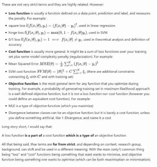
Objective function, cost function, loss function: are they the same thing?

The meaning of theta

$ h(x)=W^TX +b =\theta^Tx$

Linear regression

Hypotheses:

$$ h_\theta(x)=\theta_0+\theta_1x_1+\theta_2x_2\tag{1} $$

$$ h(x)=\sum_{i=0}^n\theta_ix_i=\theta^Tx\tag{2} $$

$$x_0 =1 $$

Loss:

$$ J(\theta)=\frac 1 2\sum_{i=1}^m(h_\theta(x^{(i)})-y^{(i)})^2\tag{3} $$

type （3） Also known as Ordinary least squares( Least square method ), and mean square error(MSE Mean square error ) Very similar , The difference lies in ：

The least square method as a loss function is not divided by the total number of samples m, Mean square error divided by the total number of samples m
The method of solving the model based on the minimization of mean square error is called “ Least square method ”.— zhou 《 machine learning 》

as for linear regression loss function Why Ordinary least square, See the link below pdf Inside Probabilistic interpretation.

Goal:

Ordinary least squares

Solutions:

Gradient descent
Normal equation

$$ \theta=(X^TX)^{-1}X^T\vec{y}\tag{4} $$

See https://see.stanford.edu/mate...

Logistic regression

Logistic function:

$$ g(z)=\frac {1} {1+e^{-z}}\tag{5} $$

$$ g'(z)=g(z)(1-g(z))\tag{6} $$

Fig.1
Pictured above Fig.1 Shown ,sigmoid The function range is 0-1, The domain of definition is R, derivative x=0 when , The maximum value is 0.25, But when x There is a risk of gradient disappearance or gradient explosion when it tends to infinity or infinity .

Hypotheses:

$$ h_\theta(x)=g(\theta^Tx)=\frac {1} {1+e^{-\theta^Tx}}\tag{7} $$

Inputting the output of linear regression into a logical function becomes logical regression , The range of values is from R Turn into 0-1, With this, we can do the task of two categories , Greater than 0.5 It's a kind of , Less than 0.5 It's a kind of .

MLE(Maximum Likelihood Estimate)

Next, from the perspective of maximum likelihood estimation to find loss function.
commonly by MLE We want to get argmax p(D$ |\theta) $, That is, finding parameters makes it possible to get such data .

Assume：

$$ P(y=1|x;\theta)=h_\theta(x)\tag{8} $$

$$ P(y=0|x;\theta)=1-h_\theta(x)\tag{9} $$

The formula （8） And the formula （9） You can synthesize formulas （10）：

$$ P(y|x;\theta)=(h_\theta(x))^y(1-h_\theta(x))^{1-y}\tag{10} $$

The formula （10） Is the likelihood probability of a sample , Also known as point estimation , So how to express the likelihood probability of the sample ？ See the following formula （11）：

Likelihood：

$$ \begin{equation}\begin{split} L(\theta)&=p(\vec{y}|X;\theta)\\ &=\prod_{i=1}^{m}p(y^{(i)}|x^{(i)};\theta)\\ &=\prod_{i=1}^{m}(h_\theta(x^{(i)}))^{y^{(i)}}(1-h_\theta(x^{(i)}))^{1-y^{(i)}}\tag{11} \end{split}\end{equation} $$

This is actually our objective function , But I want to find $ arg\,max{L(\theta)}$ We need further simplification , The simplified method is to add a log, That is to say $ log(L(\theta)) $, The advantage of this is ：

Simplify the equation , Convert continuous multiplication into continuous addition
Prevent the risk of numerical underflow in the calculation process
log It's a monotone increasing function , Will not change the nature of the original function

Log Likelihood

$$ \begin{equation}\begin{split} \ell(\theta)&=log(L(\theta))\\ &=\sum_{i=1}^{m}y^{(i)}logh_\theta(x^{(i)})+(1-y^{(i)})log(1-h_\theta(x^{(i)}))\tag{12} \end{split}\end{equation} $$

type （12） Is the maximum likelihood function we are looking for , In fact, adding a minus sign in front of it turns into Loss function, But the maximum likelihood function pursues the maximum value , and Loss function The pursuit is the minimum .

Gradient ascent for one sample:

For the convenience of derivation, I didn't put sum Add in the calculation , That is, only one sample

$$ \begin{equation}\begin{split} \frac{\partial \ell(\theta)}{\partial \theta_j}&=(y\frac{1}{g(\theta^Tx)}-(1-y)\frac{1}{1-g(\theta^Tx)})\frac{\partial g(\theta^Tx)}{\theta_j}\\ &=(y\frac{1}{g(\theta^Tx)}-(1-y)\frac{1}{1-g(\theta^Tx)})g(\theta^Tx)(1-g(\theta^Tx))\frac{\partial \theta^Tx}{\theta_j}\\ &=(y(1-g(\theta^Tx))-(1-y)g(\theta^Tx))x_j\\ &=(y-h_\theta(x))x_j\tag{13} \end{split}\end{equation} $$

so, gradient ascent rule:

$$ \theta_j:=\theta_j+\alpha(y^{(i)}-h_\theta(x)^{(i)})x_j^{(i)}\tag{14} $$