当前位置:网站首页>[hands on deep learning]02 softmax regression
[hands on deep learning]02 softmax regression
2022-07-02 20:49:00 【gokingd】
softmax Return to
1. softmax Return to
although softmax There is the word "return" in return , But in fact, this is a classification model . Similar to linear regression ,softmax Regression is a single-layer neural network , The difference is , There is only one output of linear regression , and softmax There are multiple outputs of regression .
( The picture is quoted from zh-v2.d2l.ai)
The reason softmax Regression is used for classification , Is the model passed softmax The operation converts the output into probability , Choose which category to classify according to the greater probability . Pictured above is an example , have access to o = W x + b o=Wx+b o=Wx+b Express in the form of . among W W W yes 3X4 Matrix , Each line is the weight of each parameter of the input layer to a certain classification , x x x It's the input layer , It's a 4X1 The column vector , b b b and x x x equally , Also a 4X1 The column vector , The final o o o It's a 3X1 The column vector .
Get the vector at o o o after , after softmax Operations are converted into probabilistic forms , for example [ 0.2 , 0.3 , 0.5 ] T [0.2, 0.3,0.5]^T [0.2,0.3,0.5]T, Then the sample can be classified as No 3 class .
softmax The vector expression of is very similar to linear regression ,softmax Regression is also a linear model , Even though softmax It's a nonlinear function (softmax The output of the regression is determined by the affine transformation of the input characteristics ). Often mentioned in linear models logistic Return is softmax Return to k In the classification k=2 The general form of .
2. softmax operation
First , For a given sample label x x x After affine transformation, the output o o o, Then go through softmax Function to get the prediction tag . It can be regarded as a probability distribution .
y ^ = s o f t m a x ( o ) \hat{y}=softmax(o) y^=softmax(o)
y j ^ = e x p ( o j ) ∑ k e x p ( o k ) \hat{y_j}=\frac{exp(o_j)}{\sum_kexp(o_k)} yj^=∑kexp(ok)exp(oj)
namely softmax The operation is to add up the values of the column vector , Then divide each element by the total , In this way, we can get the sum of 1, Not less than 0 In the form of probability .
Last , a r g m a x j y j ^ = a r g m a x j o j {argmax}_j\hat{y_j}=argmax_jo_j argmaxjyj^=argmaxjoj
3. Maximum likelihood estimation
Suppose the noise obeys normal distribution . In linear regression ,
y = w T x + b + ε y=w^Tx+b+\varepsilon y=wTx+b+ε
among ε ∼ N ( 0 , δ 2 ) \varepsilon\sim N(0,\delta^2) ε∼N(0,δ2)
Given x To y Likelihood function of :
P ( y ∣ x ) = 1 2 π δ 2 e x p ( − 1 2 δ 2 ( y − w T x − b ) 2 ) P(y|x)=\frac{1}{\sqrt{2\pi\delta^2}}exp(-\frac{1}{2\delta^2}(y-w^Tx-b)^2) P(y∣x)=2πδ21exp(−2δ21(y−wTx−b)2)
P ( y ∣ X ) = ∏ i = 1 n p ( y ( i ) ∣ x ( i ) ) P(y|X)=\prod^n_{i=1}p(y^{(i)}|x^{(i)}) P(y∣X)=i=1∏np(y(i)∣x(i))
To maximize the above formula , Negative log likelihood can be minimized at an equal price , You can get :
− l o g P ( y ∣ X ) = ∑ i = 1 n 1 2 l o g ( 2 π δ 2 ) + 1 2 δ 2 ( y ( i ) − w T x ( i ) − b ) -logP(y|X)=\sum^n_{i=1}\frac{1}{2}log(2\pi\delta^2)+\frac{1}{2\delta^2}(y^{(i)}-w^Tx^{(i)}-b) −logP(y∣X)=i=1∑n21log(2πδ2)+2δ21(y(i)−wTx(i)−b)
The first term is a constant term , The rest is the mean square error . That's why , Under the assumption of Gaussian noise , Minimizing the mean square error is equivalent to the maximum likelihood estimation of the linear model .
4. Loss function
Empathy , Using maximum likelihood estimation :
P ( Y ∣ X ) = ∏ i = 1 n P ( y ( i ) ∣ x ( i ) ) P(Y|X)=\prod^n_{i=1}P(y^{(i)}|x^{(i)}) P(Y∣X)=i=1∏nP(y(i)∣x(i))
Again , Minimize the negative log likelihood :
− l o g P ( Y ∣ X ) = ∑ 1 n − l o g P ( y ( i ) ∣ x ( i ) ) -logP(Y|X)=\sum^n_1-logP(y^{(i)}|x^{(i)}) −logP(Y∣X)=1∑n−logP(y(i)∣x(i))
here ,softmax Function gives the prediction vector y ^ \hat{y} y^, For each class of probability . So it can be written as , P ( y ( i ) ∣ x ( i ) ) = y ^ = ∑ j − y j l o g ( y j ^ ) P(y^{(i)}|x^{(i)})=\hat{y}=\sum_j-y_jlog(\hat{y_j}) P(y(i)∣x(i))=y^=∑j−yjlog(yj^)
Because the final label y y y yes one-hot vector , So when multiplied, there will only be one item in the end .
so : − l o g P ( Y ∣ X ) = ∑ i = 1 n ∑ j = 1 q − y i j l o g y i j ^ -logP(Y|X)=\sum_{i=1}^n\sum_{j=1}^q-y_{ij}log\hat{y_{ij}} −logP(Y∣X)=i=1∑nj=1∑q−yijlogyij^
softmax The loss function in regression is the cross entropy loss function . This is due to cross entropy loss
l ( y , y ^ ) = − ∑ j = 1 q y j l o g y j ^ l(y,\hat{y})=-\sum_{j=1}^qy_jlog\hat{y_j} l(y,y^)=−j=1∑qyjlogyj^
therefore , The final minimization of negative log likelihood can be written as :
− l o g P ( Y ∣ X ) = ∑ 1 n l l ( y ( i ) , y ^ ( i ) ) -logP(Y|X)=\sum^n_1ll(y^{(i)},\hat{y}^{(i)}) −logP(Y∣X)=1∑nll(y(i),y^(i))
Minimize the loss function .
But in the actual coding later , The loss function is usually written as :
def cross_entropy(y_hat, y):
    return - torch.log(y_hat[range(len(y_hat)), y])
This is because in the Fashion_Mnist Data set , Acquired y y y The label is not one-hot vector , It's a category .
for instance , For batch size of n, namely n A sample :
O = X W + b O=XW+b O=XW+b
Y ^ = s o f t m a x ( O ) \hat{Y}=softmax(O) Y^=softmax(O)
among X by nxd Matrix ,W by dxq Matrix ,b by 1xq Matrix , be O and y ^ \hat{y} y^ All are nxq Matrix . And obtained y The vector is nx1 Vector , Represents the classification corresponding to each sample , for example [ 2 , 3 , 1 , 0 , 5 ] T [2,3,1,0,5]^T [2,3,1,0,5]T. In the loss function , y j y_j yj Not 0 namely 1, Then only the prediction probability will be preserved log The actual value corresponding to the value is 1 The one of . This is consistent with the concept of loss function . We need to minimize the loss function , That is to maximize the prediction probability log And actual value y The product of the .
The above code is to directly take the actual value as 1 The prediction probability of that item , Retake log, The effect is the same .
5. gradient
Find the gradient of the loss function , Because the gradient descent updates the parameters in the linear network , So it's the predicted value y ^ \hat{y} y^ Derivation , Yes softmax Function o j o_j oj Derivation :
l ( y , y ^ ) = − ∑ j = 1 q y j l o g e x p ( o j ) ∑ k = 1 q e x p ( o k ) l(y,\hat{y})=-\sum^q_{j=1}y_jlog\frac{exp(o_j)}{\sum_{k=1}^qexp(o_k)} l(y,y^)=−j=1∑qyjlog∑k=1qexp(ok)exp(oj)
= ∑ j = 1 q y j l o g ∑ k = 1 q e x p ( o k ) − ∑ j = 1 q y j o j =\sum_{j=1}^qy_jlog\sum_{k=1}^qexp(o_k)-\sum_{j=1}^qy_jo_j =j=1∑qyjlogk=1∑qexp(ok)−j=1∑qyjoj
= l o g ∑ k = 1 q e x p ( o k ) − ∑ j = 1 q y j o j =log\sum_{k=1}^qexp(o_k)-\sum_{j=1}^qy_jo_j =logk=1∑qexp(ok)−j=1∑qyjoj
∂ o j l ( y , y ^ ) = e x p ( o j ) ∑ k = 1 q e x p ( o k ) − y j = s o f t m a x ( o ) j − y j \partial_{o_j}l(y,\hat{y})=\frac{exp(o_j)}{\sum_{k=1}^qexp(o_k)}-y_j=softmax(o)_j-y_j ∂ojl(y,y^)=∑k=1qexp(ok)exp(oj)−yj=softmax(o)j−yj
That is, the gradient is the observed value y y y And estimates y ^ \hat{y} y^ Differences between .
6. Realization
6.1 From zero softmax Return to
- Import related libraries and download datasets , What we use here is FashionMnist Data sets .
%matplotlib inline
import torch
import torchvision
from torch.utils import data
from torchvision import transforms
from d2l import torch as d2l
from IPython import display

d2l.use_svg_display()

trans = transforms.ToTensor()
mnist_train = torchvision.datasets.FashionMNIST(root="../data",train=True,transform=
                                               trans,download=True)
mnist_test = torchvision.datasets.FashionMNIST(root="../data",train=False,transform=trans,
                                              download=True)
- Import dataset , Train in batches
batch_size =256
def get_dataloader_workers():
    return 0
def load_data_fashion_mnist(batch_size,resize=None):
    trans = [transforms.ToTensor()]
    if resize:
        trans.insert(0,transforms.Resize(resize))
    trans = transforms.Compose(trans)
    return (data.DataLoader(mnist_train,batch_size,shuffle=True,
                            num_workers=get_dataloader_workers()),
           data.DataLoader(mnist_test,batch_size,shuffle=False,
                           num_workers=get_dataloader_workers))

batch_size= 256
train_iter,test_iter =d2l.load_data_fashion_mnist(batch_size)
there get_dataloader_workers Is the number of threads , Indicates that multiple threads can be used in parallel load data , Greater than 0 It will speed up loading .
3. Define the network model and softmax function
def softmax(X):
    X_exp = torch.exp(X)
    partition = X_exp.sum(1,keepdim=True)
    return X_exp/partition

num_inputs = 784
num_outputs = 10

W = torch.normal(0,0.01,size=(num_inputs,num_outputs),requires_grad=True)
b = torch.zeros(num_outputs,requires_grad=True)

def net(X):
    return softmax(torch.matmul(X.reshape((-1,W.shape[0])),W)+b)
- Define the loss function
def cross_entropy(y_hat,y):
    return -torch.log(y_hat[range(len(y_hat)),y])
- Define accumulation class and dynamic graph class
class Accumulator:
    def __init__(self,n):
        self.data=[0.0]*n

    def add(self,*args):
        self.data = [a+float(b) for a,b in zip(self.data,args)]

    def reset(self):
        self.data = [0.0]*len(self.data)

    def __getitem__(self,idx):
        return self.data[idx]

class Animator:
    def __init__(self,xlabel=None,ylabel=None,legend=None,xlim=None,ylim=None,
                xscale='linear',yscale='linear',fmts=('-','m--','g-','r:'),nrows=1,
                ncols=1,figsize=(3.5,2.5)):
        if legend is None:
            legend=[]
        d2l.use_svg_display()
        self.fig,self.axes = d2l.plt.subplots(nrows,ncols,figsize=figsize)
        if nrows * ncols == 1:
            self.axes = [self.axes,]
        self.config_axes = lambda:d2l.set_axes(
        self.axes[0],xlabel,ylabel,xlim,ylim,xscale,yscale,legend)
        self.X,self.Y,self.fmts = None,None,fmts

    def add(self,x,y):
        if not hasattr(y,"__len__"):
            y=[y]
        n = len(y)

        if not hasattr(x,"__len__"):
            x=[x]*n
            if not self.X:
                self.X = [[] for _ in range(n)]
            if not self.Y:
                self.Y = [[] for _ in range(n)]
        for i,(a,b) in enumerate(zip(x,y)):
            if a is not None and b is not None:
                self.X[i].append(a)
                self.Y[i].append(b)
        self.axes[0].cla()
        for x,y,fmt in zip(self.X,self.Y,self.fmts):
            self.axes[0].plot(x,y,fmt)

        self.config_axes()
        display.display(self.fig)
        display.clear_output(wait=True)
- Evaluation accuracy
def accuracy(y_hat,y):
    if len(y_hat.shape)>1 and y_hat.shape[1]>1:
        y_hat = y_hat.argmax(axis=1)
    cmp = y_hat.type(y.dtype)==y
    return float(cmp.type(y.dtype).sum())
def evaluate_accuracy(net,data_iter):
    if isinstance(net,torch.nn.Module):
        net.eval()
    metric = Accumulator(2)
    for X,y in data_iter:
        metric.add(accuracy(net(X),y),y.numel())
    return metric[0]/metric[1]
- Gradient descent for training
def train_epoch_ch3(net,train_iter,loss,updater):
    if isinstance(net,torch.nn.Module):
        net.train()
    metric = Accumulator(3)
    for X,y in train_iter:
        y_hat = net(X)
        l = loss(y_hat,y)
        if isinstance(updater,torch.optim.Optimizer):
            updater.zero_grad()
            l.mean().backward()
            updater.step()
        else:
            l.sum().backward()
            updater(X.shape[0])
        metric.add(float(l.sum()),accuracy(y_hat,y),y.numel())

    return metric[0]/metric[2],metric[1]/metric[2]

def train_ch3(net,train_iter,test_iter,loss,num_epochs,updater):
    animator = Animator(xlabel='epoch',xlim=[1,num_epochs],ylim=[0.3,0.9],
                       legend=['train_loss','train acc','test acc'])
    for epoch in range(num_epochs):
        train_metrics = train_epoch_ch3(net,train_iter,loss,updater)
        test_acc = evaluate_accuracy(net,test_iter)
        animator.add(epoch+1,train_metrics+(test_acc,))
    train_loss , train_acc = train_metrics
    assert train_loss <0.5 ,train_loss
    assert train_acc <=1 and train_acc >0.7 , train_acc
    assert test_acc <=1 and test_acc > 0.7 , test_acc
- Finally, the random gradient descent used before is used for parameter training
lr = 0.1
def updater(batch_size):
    return d2l.sgd([W,b],lr,batch_size)
num_epochs =10
train_ch3(net,train_iter,test_iter,cross_entropy,num_epochs,updater)

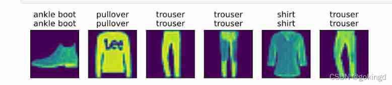
9. The trained model can be used for prediction
def predict_ch3(net,test_iterm,n=6):
for X,y in test_iter:
break
trues = d2l.get_fashion_mnist_labels(y)
preds = d2l.get_fashion_mnist_labels(net(X).argmax(axis=1))
titles=[true + ‘\n’ + pred for true,pred in zip(trues,preds)]
d2l.show_images(X[0:n].reshape((n,28,28)),1,n,titles=titles[0:n])
predict_ch3(net,test_iter)
6.2 Concise implementation
7. After-school exercises
Reference
https://zh-v2.d2l.ai/
边栏推荐
- Don't you want to have a face-to-face communication with cloud native and open source experts? (including benefits
- JASMINER X4 1U deep disassembly reveals the secret behind high efficiency and power saving
- Friends who firmly believe that human memory is stored in macromolecular substances, please take a look
- Research Report on the overall scale, major manufacturers, major regions, products and application segmentation of precoated metallic coatings in the global market in 2022
- Cs5268 perfectly replaces ag9321mcq typec multi in one docking station solution
- [error record] the command line creates an error pub get failed (server unavailable) -- attempting retry 1 in 1 second
- When Valentine's Day falls on Monday
- Properties of expectation and variance
- Interpretation of some papers published by Tencent multimedia laboratory in 2021
- [JS] get the search parameters of URL in hash mode
猜你喜欢

Complete example of pytorch model saving +does pytorch model saving only save trainable parameters? Yes (+ solution)

How to realize the function of detecting browser type in Web System
![[fluent] dart technique (independent main function entry | nullable type determination | default value setting)](/img/cc/3e4ff5cb2237c0f2007c61db1c346d.jpg)
[fluent] dart technique (independent main function entry | nullable type determination | default value setting)
SBT tutorial
![[internship] solve the problem of too long request parameters](/img/42/413cf867f0cb34eeaf999f654bf02f.png)
[internship] solve the problem of too long request parameters
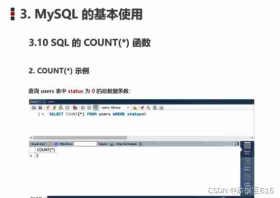
Basic concept of database, installation and configuration of database, basic use of MySQL, operation of database in the project

ROS learning (10): ROS records multiple topic scripts

通信人的经典语录,第一条就扎心了……

Resunet tensorrt8.2 speed and video memory record table on Jetson Xavier NX (continuously supplemented later)
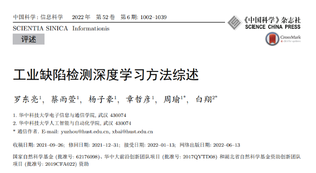
Review of the latest 2022 research on "deep learning methods for industrial defect detection"
随机推荐
Complete example of pytorch model saving +does pytorch model saving only save trainable parameters? Yes (+ solution)
Research Report on the overall scale, major manufacturers, major regions, products and applications of outdoor vacuum circuit breakers in the global market in 2022
Basic concept of database, installation and configuration of database, basic use of MySQL, operation of database in the project
Resunnet - tensorrt8.2 Speed and Display record Sheet on Jetson Xavier NX (continuously supplemented)
Second hand housing data analysis and prediction system
【实习】解决请求参数过长问题
Research Report on the overall scale, major manufacturers, major regions, products and application segmentation of power management units in the global market in 2022
Happy Lantern Festival! Tengyuanhu made you a bowl of hot dumplings!
AMD's largest transaction ever, the successful acquisition of Xilinx with us $35billion
How to do interface testing? After reading this article, it will be clear
Research Report on the overall scale, major manufacturers, major regions, products and application segmentation of precoated metallic coatings in the global market in 2022
Exemple complet d'enregistrement du modèle pytoch + enregistrement du modèle pytoch seuls les paramètres d'entraînement sont - ils enregistrés? Oui (+ Solution)
SBT tutorial
Attack and defense world PWN question: Echo
数据库模式笔记 --- 如何在开发中选择合适的数据库+关系型数据库是谁发明的?
Interpretation of some papers published by Tencent multimedia laboratory in 2021
1007 maximum subsequence sum (25 points) "PTA class a exercise"
Sword finger offer (II) -- search in two-dimensional array
想请教一下,究竟有哪些劵商推荐?手机开户是安全么?
Research Report on the overall scale, major manufacturers, major regions, products and applications of swivel chair gas springs in the global market in 2022