当前位置:网站首页>ML之shap:基于adult人口普查收入二分类预测数据集(预测年收入是否超过50k)利用shap决策图结合LightGBM模型实现异常值检测案例之详细攻略
ML之shap:基于adult人口普查收入二分类预测数据集(预测年收入是否超过50k)利用shap决策图结合LightGBM模型实现异常值检测案例之详细攻略
2022-07-07 00:33:00 【一个处女座的程序猿】
ML之shap:基于adult人口普查收入二分类预测数据集(预测年收入是否超过50k)利用shap决策图结合LightGBM模型实现异常值检测案例之详细攻略
目录
基于adult人口普查收入二分类预测数据集(预测年收入是否超过50k)利用shap决策图结合LightGBM模型实现异常值检测案例之详细攻略
相关文章
ML之shap:基于adult人口普查收入二分类预测数据集(预测年收入是否超过50k)利用shap决策图结合LightGBM模型实现异常值检测案例之详细攻略
ML之shap:基于adult人口普查收入二分类预测数据集(预测年收入是否超过50k)利用shap决策图结合LightGBM模型实现异常值检测案例之详细攻略实现
基于adult人口普查收入二分类预测数据集(预测年收入是否超过50k)利用shap决策图结合LightGBM模型实现异常值检测案例之详细攻略
# 1、定义数据集
| age | workclass | fnlwgt | education | education_num | marital_status | occupation | relationship | race | sex | capital_gain | capital_loss | hours_per_week | native_country | salary |
| 39 | State-gov | 77516 | Bachelors | 13 | Never-married | Adm-clerical | Not-in-family | White | Male | 2174 | 0 | 40 | United-States | <=50K |
| 50 | Self-emp-not-inc | 83311 | Bachelors | 13 | Married-civ-spouse | Exec-managerial | Husband | White | Male | 0 | 0 | 13 | United-States | <=50K |
| 38 | Private | 215646 | HS-grad | 9 | Divorced | Handlers-cleaners | Not-in-family | White | Male | 0 | 0 | 40 | United-States | <=50K |
| 53 | Private | 234721 | 11th | 7 | Married-civ-spouse | Handlers-cleaners | Husband | Black | Male | 0 | 0 | 40 | United-States | <=50K |
| 28 | Private | 338409 | Bachelors | 13 | Married-civ-spouse | Prof-specialty | Wife | Black | Female | 0 | 0 | 40 | Cuba | <=50K |
| 37 | Private | 284582 | Masters | 14 | Married-civ-spouse | Exec-managerial | Wife | White | Female | 0 | 0 | 40 | United-States | <=50K |
| 49 | Private | 160187 | 9th | 5 | Married-spouse-absent | Other-service | Not-in-family | Black | Female | 0 | 0 | 16 | Jamaica | <=50K |
| 52 | Self-emp-not-inc | 209642 | HS-grad | 9 | Married-civ-spouse | Exec-managerial | Husband | White | Male | 0 | 0 | 45 | United-States | >50K |
| 31 | Private | 45781 | Masters | 14 | Never-married | Prof-specialty | Not-in-family | White | Female | 14084 | 0 | 50 | United-States | >50K |
| 42 | Private | 159449 | Bachelors | 13 | Married-civ-spouse | Exec-managerial | Husband | White | Male | 5178 | 0 | 40 | United-States | >50K |
# 2、数据集预处理
# 2.1、入模特征初步筛选
df.columns
14
# 2.2、目标特征二值化
# 2.3、类别型特征编码数字化
| age | workclass | education_num | marital_status | occupation | relationship | race | sex | capital_gain | capital_loss | hours_per_week | native_country | salary | |
| 0 | 39 | 7 | 13 | 4 | 1 | 1 | 4 | 1 | 2174 | 0 | 40 | 39 | 0 |
| 1 | 50 | 6 | 13 | 2 | 4 | 0 | 4 | 1 | 0 | 0 | 13 | 39 | 0 |
| 2 | 38 | 4 | 9 | 0 | 6 | 1 | 4 | 1 | 0 | 0 | 40 | 39 | 0 |
| 3 | 53 | 4 | 7 | 2 | 6 | 0 | 2 | 1 | 0 | 0 | 40 | 39 | 0 |
| 4 | 28 | 4 | 13 | 2 | 10 | 5 | 2 | 0 | 0 | 0 | 40 | 5 | 0 |
| 5 | 37 | 4 | 14 | 2 | 4 | 5 | 4 | 0 | 0 | 0 | 40 | 39 | 0 |
| 6 | 49 | 4 | 5 | 3 | 8 | 1 | 2 | 0 | 0 | 0 | 16 | 23 | 0 |
| 7 | 52 | 6 | 9 | 2 | 4 | 0 | 4 | 1 | 0 | 0 | 45 | 39 | 1 |
| 8 | 31 | 4 | 14 | 4 | 10 | 1 | 4 | 0 | 14084 | 0 | 50 | 39 | 1 |
| 9 | 42 | 4 | 13 | 2 | 4 | 0 | 4 | 1 | 5178 | 0 | 40 | 39 | 1 |
# 2.4、分离特征与标签
| age | workclass | education_num | marital_status | occupation | relationship | race | sex | capital_gain | capital_loss | hours_per_week | native_country |
| 39 | 7 | 13 | 4 | 1 | 1 | 4 | 1 | 2174 | 0 | 40 | 39 |
| 50 | 6 | 13 | 2 | 4 | 0 | 4 | 1 | 0 | 0 | 13 | 39 |
| 38 | 4 | 9 | 0 | 6 | 1 | 4 | 1 | 0 | 0 | 40 | 39 |
| 53 | 4 | 7 | 2 | 6 | 0 | 2 | 1 | 0 | 0 | 40 | 39 |
| 28 | 4 | 13 | 2 | 10 | 5 | 2 | 0 | 0 | 0 | 40 | 5 |
| 37 | 4 | 14 | 2 | 4 | 5 | 4 | 0 | 0 | 0 | 40 | 39 |
| 49 | 4 | 5 | 3 | 8 | 1 | 2 | 0 | 0 | 0 | 16 | 23 |
| 52 | 6 | 9 | 2 | 4 | 0 | 4 | 1 | 0 | 0 | 45 | 39 |
| 31 | 4 | 14 | 4 | 10 | 1 | 4 | 0 | 14084 | 0 | 50 | 39 |
| 42 | 4 | 13 | 2 | 4 | 0 | 4 | 1 | 5178 | 0 | 40 | 39 |
| salary |
| 0 |
| 0 |
| 0 |
| 0 |
| 0 |
| 0 |
| 0 |
| 1 |
| 1 |
| 1 |
#3、模型训练与推理
# 3.1、数据集切分
X_test
| age | workclass | education_num | marital_status | occupation | relationship | race | sex | capital_gain | capital_loss | hours_per_week | native_country | |
| 1342 | 47 | 3 | 10 | 0 | 1 | 1 | 4 | 1 | 0 | 0 | 40 | 35 |
| 1338 | 71 | 3 | 13 | 0 | 13 | 3 | 4 | 0 | 2329 | 0 | 16 | 35 |
| 189 | 58 | 6 | 16 | 2 | 10 | 0 | 4 | 1 | 0 | 0 | 1 | 35 |
| 1332 | 23 | 3 | 9 | 4 | 7 | 1 | 2 | 1 | 0 | 0 | 35 | 35 |
| 1816 | 46 | 2 | 9 | 2 | 3 | 0 | 4 | 1 | 0 | 1902 | 40 | 35 |
| 1685 | 37 | 3 | 9 | 2 | 4 | 0 | 4 | 1 | 0 | 1902 | 45 | 35 |
| 657 | 34 | 3 | 9 | 2 | 3 | 0 | 4 | 1 | 0 | 0 | 45 | 35 |
| 1846 | 21 | 0 | 10 | 4 | 0 | 3 | 4 | 0 | 0 | 0 | 40 | 35 |
| 554 | 33 | 1 | 11 | 0 | 3 | 4 | 2 | 0 | 0 | 0 | 40 | 35 |
| 1963 | 49 | 3 | 13 | 2 | 12 | 0 | 4 | 1 | 0 | 0 | 50 | 35 |
# 3.2、模型建立并训练
params = {
    "max_bin": 512, "learning_rate": 0.05,
    "boosting_type": "gbdt", "objective": "binary",
    "metric": "binary_logloss", "verbose": -1,
     "min_data": 100, "random_state": 1,
    "boost_from_average": True, "num_leaves": 10 }

LGBMC = lgb.train(params, lgbD_train, 10000,
                  valid_sets=[lgbD_test],
                  early_stopping_rounds=50,
                  verbose_eval=1000)
# 3.3、模型预测
| age | workclass | education_num | marital_status | occupation | relationship | race | sex | capital_gain | capital_loss | hours_per_week | native_country | y_test_predi | y_test | |
| 1342 | 47 | 3 | 10 | 0 | 1 | 1 | 4 | 1 | 0 | 0 | 40 | 35 | 0.045225575 | 0 |
| 1338 | 71 | 3 | 13 | 0 | 13 | 3 | 4 | 0 | 2329 | 0 | 16 | 35 | 0.074799172 | 0 |
| 189 | 58 | 6 | 16 | 2 | 10 | 0 | 4 | 1 | 0 | 0 | 1 | 35 | 0.30014332 | 1 |
| 1332 | 23 | 3 | 9 | 4 | 7 | 1 | 2 | 1 | 0 | 0 | 35 | 35 | 0.003966427 | 0 |
| 1816 | 46 | 2 | 9 | 2 | 3 | 0 | 4 | 1 | 0 | 1902 | 40 | 35 | 0.363861294 | 0 |
| 1685 | 37 | 3 | 9 | 2 | 4 | 0 | 4 | 1 | 0 | 1902 | 45 | 35 | 0.738628671 | 1 |
| 657 | 34 | 3 | 9 | 2 | 3 | 0 | 4 | 1 | 0 | 0 | 45 | 35 | 0.376412174 | 0 |
| 1846 | 21 | 0 | 10 | 4 | 0 | 3 | 4 | 0 | 0 | 0 | 40 | 35 | 0.002309884 | 0 |
| 554 | 33 | 1 | 11 | 0 | 3 | 4 | 2 | 0 | 0 | 0 | 40 | 35 | 0.060345836 | 1 |
| 1963 | 49 | 3 | 13 | 2 | 12 | 0 | 4 | 1 | 0 | 0 | 50 | 35 | 0.703506366 | 1 |
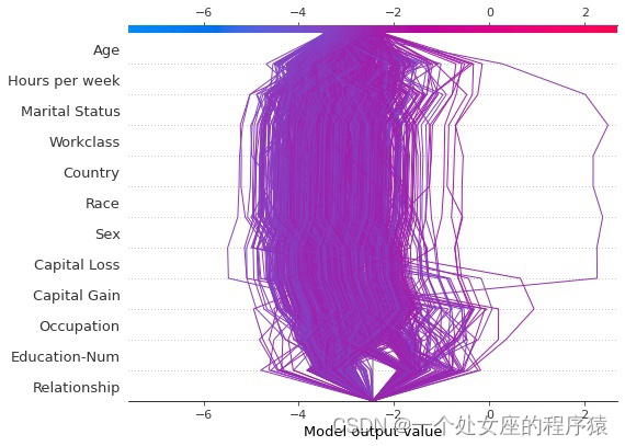
# 4、利用shap决策图进行异常值检测
# 4.1、原始数据和预处理后的数据各采样一小部分样本
# 4.2、创建Explainer并计算SHAP值
shap2exp.values.shape (100, 12, 2)
 [[[-5.97178729e-01  5.97178729e-01]
  [-5.18879297e-03  5.18879297e-03]
  [ 1.70566444e-01 -1.70566444e-01]
  ...
  [ 0.00000000e+00  0.00000000e+00]
  [ 6.58794799e-02 -6.58794799e-02]
  [ 0.00000000e+00  0.00000000e+00]]

 [[-4.45574118e-01  4.45574118e-01]
  [-1.00665452e-03  1.00665452e-03]
  [-8.12237233e-01  8.12237233e-01]
  ...
  [ 0.00000000e+00  0.00000000e+00]
  [ 8.56381961e-01 -8.56381961e-01]
  [ 0.00000000e+00  0.00000000e+00]]

 [[-3.87412165e-01  3.87412165e-01]
  [ 1.52848351e-01 -1.52848351e-01]
  [-1.02755954e+00  1.02755954e+00]
  ...
  [ 0.00000000e+00  0.00000000e+00]
  [ 1.10240434e+00 -1.10240434e+00]
  [ 0.00000000e+00  0.00000000e+00]]

 ...

 [[-5.28928223e-01  5.28928223e-01]
  [ 7.14116015e-03 -7.14116015e-03]
  [-8.82241728e-01  8.82241728e-01]
  ...
  [ 0.00000000e+00  0.00000000e+00]
  [ 7.47521189e-02 -7.47521189e-02]
  [ 0.00000000e+00  0.00000000e+00]]

 [[ 2.20002984e+00 -2.20002984e+00]
  [ 7.75916086e-03 -7.75916086e-03]
  [ 3.95152810e-01 -3.95152810e-01]
  ...
  [ 0.00000000e+00  0.00000000e+00]
  [ 1.52566789e-01 -1.52566789e-01]
  [ 0.00000000e+00  0.00000000e+00]]

 [[-8.28965461e-01  8.28965461e-01]
  [-4.43687947e-02  4.43687947e-02]
  [ 3.37305776e-01 -3.37305776e-01]
  ...
  [ 0.00000000e+00  0.00000000e+00]
  [ 8.26477289e-03 -8.26477289e-03]
  [ 0.00000000e+00  0.00000000e+00]]]
shap2array.shape (100, 12)
LightGBM binary classifier with TreeExplainer shap values output has changed to a list of ndarray
 [[ 5.97178729e-01  5.18879297e-03 -1.70566444e-01 ...  0.00000000e+00
  -6.58794799e-02  0.00000000e+00]
 [ 4.45574118e-01  1.00665452e-03  8.12237233e-01 ...  0.00000000e+00
  -8.56381961e-01  0.00000000e+00]
 [ 3.87412165e-01 -1.52848351e-01  1.02755954e+00 ...  0.00000000e+00
  -1.10240434e+00  0.00000000e+00]
 ...
 [ 5.28928223e-01 -7.14116015e-03  8.82241728e-01 ...  0.00000000e+00
  -7.47521189e-02  0.00000000e+00]
 [-2.20002984e+00 -7.75916086e-03 -3.95152810e-01 ...  0.00000000e+00
  -1.52566789e-01  0.00000000e+00]
 [ 8.28965461e-01  4.43687947e-02 -3.37305776e-01 ...  0.00000000e+00
  -8.26477289e-03  0.00000000e+00]]
mode_exp_value: -1.9982244224656025
# 4.3、shap决策图可视化
# 将决策图叠加在一起有助于根据shap定位异常值,即偏离密集群处的样本
边栏推荐
- 【Shell】清理nohup.out文件
- Codeforces Round #416 (Div. 2) D. Vladik and Favorite Game
- 微信小程序蓝牙连接硬件设备并进行通讯,小程序蓝牙因距离异常断开自动重连,js实现crc校验位
- Message queue: how to handle repeated messages?
- Polynomial locus of order 5
- Reading notes of Clickhouse principle analysis and Application Practice (6)
- Hcip eighth operation
- PTA 天梯赛练习题集 L2-002 链表去重
- PowerPivot——DAX(函数)
- SAP ABAP BDC(批量数据通信)-018
猜你喜欢
EMMC打印cqhci: timeout for tag 10提示分析与解决
What are the common message queues?
2pc of distributed transaction solution
Cve-2021-3156 vulnerability recurrence notes
集群、分布式、微服務的區別和介紹

I didn't know it until I graduated -- the principle of HowNet duplication check and examples of weight reduction
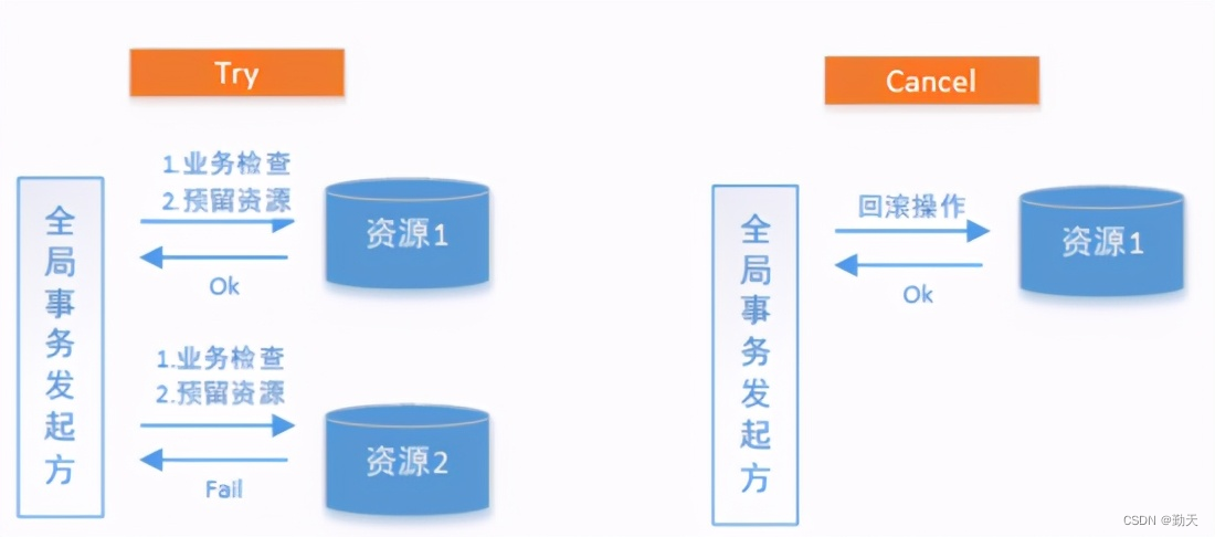
分布式事务解决方案之TCC
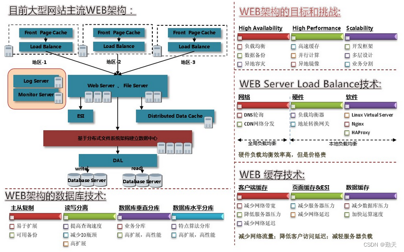
Web architecture design process

How to improve website weight
Web authentication API compatible version information
随机推荐
什么是消息队列?
集群、分布式、微服務的區別和介紹
Get the way to optimize the one-stop worktable of customer service
Randomly generate session_ id
数字IC面试总结(大厂面试经验分享)
Industrial Finance 3.0: financial technology of "dredging blood vessels"
Web architecture design process
Pinduoduo product details interface, pinduoduo product basic information, pinduoduo product attribute interface
On the difference between FPGA and ASIC
[reading of the paper] a multi branch hybrid transformer network for channel terminal cell segmentation
English grammar_ Noun possessive
nodejs获取客户端ip
How to get free traffic in pinduoduo new store and what links need to be optimized in order to effectively improve the free traffic in the store
I didn't know it until I graduated -- the principle of HowNet duplication check and examples of weight reduction
Taobao Commodity details page API interface, Taobao Commodity List API interface, Taobao Commodity sales API interface, Taobao app details API interface, Taobao details API interface
What is dependency injection (DI)
毕业之后才知道的——知网查重原理以及降重举例
mac版php装xdebug环境(m1版)
Realize GDB remote debugging function between different network segments
An example of multi module collaboration based on NCF