Simple demo of solving BP neural network by gradient descent method

  Original article , Reprint please indicate from 《 Old cake explains neural networks 》:bp.bbbdata.com

About 《 Old cake explains neural networks 》：

This website structurally explains the knowledge of Neural Networks , Principle and code .

repeat matlab Algorithm of neural network toolbox , It is a good assistant for learning neural networks . 

---

Catalog

One 、BP Model is introduced

01.BP Structure and bionic thinking of   

02.  frequently-used BP structure   

03. BP The mathematical structure of （ expression ） 

Two 、 The gradient descent method is used to solve the problem BP neural network

01 .  problem

02.  Modeling ideas   

03.  Code implementation   

04.  Running results   

05.  Test the effect of the model

---

The first part of this article introduces BP Model structure and mathematical expression of neural network ,

The second part introduces the gradient descent method to solve BP Specific examples and codes of Neural Networks （ Does not rely on any third party packages ）.

The layout is messy , No longer adjust , If you need it, you can check it directly on the original network .

One 、BP Model is introduced

---

  01.BP Structure and bionic thinking of   

BP The idea is to imitate the working principle of human brain , Construct a mathematical model ,

Its bionic structure is as follows （ Also known as BP Neural network topology ）

     structure      

its   The structure consists of three layers , The top one is the input layer , In the middle is the hidden layer （ There can be multiple hidden layers , Each hidden layer can have multiple neurons ）, Finally, the output layer .

   Workflow   

(1)  The input layer is responsible for receiving input , After the input layer receives the input , Each input neuron will transfer the value weight to each hidden layer neuron ,
(2)  Each hidden neuron receives the value transmitted by the input neuron , With its own basic threshold b Summation summation , After an activation function （ Usually the activation function is tansig function ）, Then the weighting is transmitted to the output layer .
(3)  The output neuron compares the value transmitted by each hidden neuron with its own threshold b Sum up （ After summation, it can also go through another layer of transformation ）, That is, the output value .

   Bionic principle   

---

See symbols in your eyes “5” After , The brain will recognize that it is 5.BP It is to imitate this behavior . This behavior process is simply divided into ： 
  (1)   The eyes accept the input                     
  (2)   Transmit input signals to other brain neurons         
  (3)   After comprehensive processing of brain neurons , The output is 5   
We all know ,  Neurons transmit values in the mode of nerve impulse , The signal reaches the neuron , All exist in the form of electrical signals ,
When electrical signals accumulate in neurons above the threshold , Will trigger nerve impulses , Transmit electrical signals to other neurons .                                 
According to this principle , The above neural network structure is constructed .    

 02.  frequently-used BP structure   

---

Above is the general structure , Number of hidden layers 、 Activation functions are undetermined .

Most commonly used , Is to set a hidden layer ,

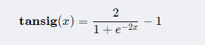
The activation function of hidden layer neurons is set to tansig function ,

The activation function of the output layer is set to purelin

In this way , The structure is shown in the figure below ：

among ,
tansig Function is S Type of function ： 

purelin  Is an identical linear mapping function ：     

PASS:
1、 The output layer is set to purelin, That is, there is no active function in the output layer .
2、  The hidden layer activation function can also be set to logsig  : , It and tansig There are not many qualitative differences . The difference lies in ,logsig The range of phi is zero 【0,1】, and tansig yes 【-1,1】.

   03. BP The mathematical structure of （ expression ） 

---

ad locum , We do not provide a general mathematical structure ,

Just take a simple example , Tell about its mathematical structure , This is more specific and easy to understand .

There is one BP neural network , Its structure is as follows :

---

1、 An input layer , A hidden layer , An output layer ,  Input layer 、 Cryptic layer 、 The number of nodes in the output layer is  [2 ,3,1].
2、 Transfer function settings ： Cryptic layer （ tansig function ）. Output layer （purelin function ）.                                           

---

The model topology is as follows ：

---

---

The mathematical expression can be written according to the model as follows ：

---

PASS:  There are many parameters in the expression , But there are only two types of parameters ： The weight w And thresholds b.              
Representing this weight is the... Th 2 Layer of the first 2 Nodes to 3 Layer of the first 1 Weight of nodes .         
This threshold is the second 2 Layer of the first 1 Threshold of nodes .                                          
remarks ： Weight matrices w The subscript , Generally from the back layer to the front layer , This is more concise in matrix expression     

---

Two 、 The gradient descent method is used to solve the problem BP neural network

---

01 .  problem

---

The following data are available ：

y It's actually from  ​ Generate

Now? , We need to train a neural network , Fit it , Last , We'll talk to Compare

  02.  Modeling ideas   

---

   Set up neural network structure   

Here we set it as a hidden layer ,3 Hidden neurons , The hidden layer activation function is tansig,

Then our network topology is as follows ：
 

 
The mathematical expression of the corresponding model is :

   Loss function and gradient   

---

The loss function is ：

---

Cryptic layer --> The weight of the output layer 、 The threshold gradient of the output layer is ：





among , Is the activation value of the hidden layer ,         

Is the node gradient of the output layer ：

---

Cryptic layer --> The weight of the output layer 、 The threshold gradient of the hidden layer is ：





among , Is the node gradient of the hidden layer ：

---

    count   Law   flow   cheng    

---

Initialize first W,b,
(1)  Calculate the gradient according to the gradient formula
(2)  take W Adjust in the direction of negative gradient
Keep cycling (1) and (2), Until the termination conditions are met ( For example, the maximum number of iterations is reached , Or the error is small enough )

  03.  Code implementation   

---

---

close all;clear all;
%----------- data ----------------------
x1 = [-3,-2.7,-2.4,-2.1,-1.8,-1.5,-1.2,-0.9,-0.6,-0.3,0,0.3,0.6,0.9,1.2,1.5,1.8];% x1：x1 = -3:0.3:2;
x2 = [-2,-1.8,-1.6,-1.4,-1.2,-1,-0.8,-0.6,-0.4,-0.2,-2.2204,0.2,0.4,0.6,0.8,1,1.2]; % x2：x2 = -2:0.2:1.2;
X  = [x1;x2];      %  take x1,x2 As input data 
y  = [0.6589,0.2206,-0.1635,-0.4712,-0.6858,-0.7975,-0.8040,...
    -0.7113,-0.5326,-0.2875 ,0.9860,0.3035,0.5966,0.8553,1.0600,1.1975,1.2618];    % y： y = sin(x1)+0.2*x2.*x2;

%-------- Parameter setting and constant calculation -------------
setdemorandstream(88);
hide_num = 3;
lr = 0.05;
[in_num,sample_num] = size(X);
[out_num,~] =  size(y);

%-------- initialization w,b And forecast results -----------
w_ho = rand(out_num,hide_num);   %  Weight from hidden layer to output layer  
b_o  = rand(out_num,1);          %  Output layer threshold 
w_ih = rand(hide_num,in_num);    %  Input layer to hidden layer weight 
b_h  = rand(hide_num,1);         %  Hidden layer threshold 
simy = w_ho*tansig(w_ih*X+repmat(b_h,1,size(X,2)))+repmat(b_o,1,size(X,2)); %  Predicted results 
mse_record = [sum(sum((simy - y ).^2))/(sample_num*out_num)];  %  Prediction error record 

% --------- Training with gradient descent ------------------
for i = 1:5000
    % Calculate the gradient 
    hide_Ac = tansig(w_ih*X+repmat(b_h,1,sample_num)); %  Hidden node activation value 
    dNo     = 2*(simy - y )/(sample_num*out_num);      %  Output layer node gradient 
    dw_ho   = dNo*hide_Ac';                            %  Cryptic layer - Output layer weight gradient 
    db_o    = sum(dNo,2);                              %  Output layer threshold gradient 
    
    dNh     = (w_ho'*dNo).*(1-hide_Ac.^2);             %  Hidden layer node gradient 
    dw_ih   = dNh*X';                                  %  Input layer - Hidden layer weight gradient 
    db_h    = sum(dNh,2);                              %  Hidden layer threshold gradient 

    % Update to a negative gradient w,b
    w_ho = w_ho - lr*dw_ho;                            %  Update hidden layer - Output layer weight  
    b_o  = b_o  - lr*db_o;                             %  Update the output layer threshold 
    w_ih = w_ih - lr*dw_ih;                            %  Update input layer - Hidden layer weight  
    b_h  = b_h  - lr*db_h;                             %  Update hidden layer threshold 
    
    %  Calculate the network prediction results and record errors 
    simy = w_ho*tansig(w_ih*X+repmat(b_h,1,size(X,2)))+repmat(b_o,1,size(X,2));
    mse_record =[mse_record, sum(sum((simy - y ).^2))/(sample_num*out_num)];
end

% ------------- Draw training results and print model parameters -----------------------------
h = figure;
subplot(1,2,1)
plot(mse_record)
subplot(1,2,2)
plot(1:sample_num,y);
hold on
plot(1:sample_num,simy,'-r');
set(h,'units','normalized','position',[0.1 0.1 0.8 0.5]);
%-- Model parameters --
w_ho   %  Weight from hidden layer to output layer  
b_o    %  Output layer threshold 
w_ih   %  Input layer to hidden layer weight 
b_h    %  Hidden layer threshold 

 04.  Running results   

---

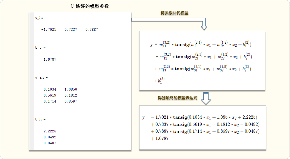
05.  Test the effect of the model

---

Use x =[0.5,0.5] To test , 

   Model predictions    

---

take  x =[0.5,0.5]  Substitute the above network model expression , obtain  0.6241

---

   The real result    

---

take  x =[0.5,0.5]  Substitute real relationships     Get in 0.5294 .

---

   Analysis of prediction results    

---

The predicted value of the network 0.6241 And the real value 0.5294  error 0.0946.
This error is not too big , But it's not small .
As a whole , Model training has certain effect , It shows that the algorithm is feasible .
 PASS: Why is the training data so good , There is still such a big gap in the predicted value ？ Can readers figure it out ？ Can it be improved ？ How can we improve ？

---

important clause ： The realization of the whole solution process of the above gradient descent method , It's very rough , Just as a reference for getting started .

---

Related articles

​《BP Neural network gradient derivation 》

​​​​​​《BP The mathematical expression extracted by neural network 》

《 One BP Complete modeling process 》