基于谱加权的波束方向图分析

谱加权

   本篇文章主要分析线列阵，下式给出了$u$空间的波束方向图的推导公式
$$B_u(u)={\omega }^H{v}_u(u)=e^{-j\frac{N-1}{2}\frac{2\pi d}{\lambda }u}\sum _{n=0}^{N-1}{\omega }_n^{\ast }{e}^{jn\frac{2\pi d}{\lambda }u}$$
   我们可以看到，波束方向图是权值与流形矢量的数量积，本篇文章主要分析不同的权值对波束方向图产生的不同影响，因为以下考虑的权值全部为实对称的，所以可以把n个阵元的位置用下面的标号代替$$\tilde{n}=n-\frac{N-1}{2}，n=0,1,\cdots ,N-1$$

cosine加权

   考虑N为奇数的情况，cosine的权值为$$\omega (\tilde{n})=sin(\frac{\pi }{2N})cos(\pi \frac{\tilde{n}}{N}),-\frac{N-1}{2}\le \tilde{n}\le \frac{N-1}{2}$$
其中$sin(\frac{\pi }{2N})$是一个常数，目的是为了是的$B_u(0)=1,把cosine写成指数形式，逐步变形最终可以得到$
$$B_u(u)=\frac{1}{2}sin(\frac{\pi }{2N})\{\frac{sin(\frac{N\pi }{2}(u-\frac{1}{N}))}{sin(\frac{\pi }{2}(u-\frac{1}{N}))}+\frac{sin(\frac{N\pi }{2}(u+\frac{1}{N}))}{sin(\frac{\pi }{2}(u+\frac{1}{N}))}\}$$
我们可以直接利用计算机的计算能力，让其帮助我们处理权值与流形矢量的乘积，下面给出结果

我们可以看到旁瓣变得更低，而主瓣也变宽了，下面看一下各项数据的对比

matlab代码

clear all
close all

M=11;
d=0.5;              % sensor spacing wrt wavelength
D = [-(M-1)/2:1:(M-1)/2]*d; % sensor positions in wavelengths
% weights, normalized so that w(0)=1
W_unf = ones(1,M);
W_cos = cos(pi*D*2/M);

% Beampatterns 
u = [0:0.001:1];              
A = exp(-j*2*pi*D.'*u);
G_unf = W_unf*A;
G_unf = G_unf/(max(abs(G_unf)));
G_cos = W_cos*A;
G_cos = G_cos/(max(abs(G_cos)));
figure
% array only
clf
plot(u,20*log10(abs(G_unf)),'--')
hold on
plot(u,20*log10(abs(G_cos)),'-')
hold off
axis([0 1 -80 0])
%title([int2str(M) ' element array'])
h=legend('Uniform','Cosine');
set(h,'Fontsize',12)
xlabel('\it u','Fontsize',14)
ylabel('Beam pattern (dB)','Fontsize',14)

升余弦加权

   权值$$\omega (\tilde{n})=c(p)(p+(1-p)cos(\pi \frac{\tilde{n}}{N})),\tilde{n}=-\frac{N-1}{2},\cdots ,\frac{N-1}{2}$$
其中$c(p)$是一个常数，使得$B_u(0)=1$$$c(p)=\frac{p}{N}+\frac{(1-p)}{2}sin(\frac{\pi }{2N})$$
下图给出了$p=0.31,0.17,0$时的波束方向图


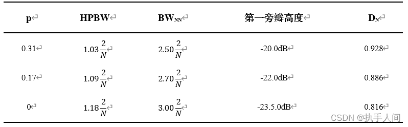
当$p$减小时，第一旁瓣的高度减小，主波束宽度增加，所以我们已经可以使得HPBW变窄，并使得第一旁瓣比均匀分布的情况要低得多

matlab代码

clear all
close all

M=11;
d=0.5;             % sensor spacing wrt wavelength
D = [-(M-1)/2:1:(M-1)/2]*d; % sensor positions in wavelengths

% weights, normalized so that w(0)=1
p=[0;0.17;0.31;1];
W_rcos = p*ones(1,M)+(ones(4,1)-p)*cos(pi*D*2/M);

% Beampatterns
u = [0:0.001:1];
c=p+(ones(4,1)-p)*2/pi;
A = exp(-j*2*pi*D.'*u);
G_rcos = W_rcos*A;
for m=1:4
 G_rcos(m,:) = G_rcos(m,:)/(max(abs(G_rcos(m,:))));
end

figure
clf
plot(u,20*log10(abs(G_rcos(3,:))),'-.')
hold on
plot(u,20*log10(abs(G_rcos(2,:))),'--')
plot(u,20*log10(abs(G_rcos(1,:))),'-')
hold off
axis([0 1 -80 0])
h=legend('{\it p}=0.31','{\it p}=0.17','{\it p}=0');
set(h,'Fontsize',12)
xlabel('\it u','Fontsize',14)
ylabel('Beam pattern (dB)','Fontsize',14)

cosine^m加权

下面分析一系列cosine加权，形成$co{s}^m(\frac{\pi \tilde{n}}{N})$，z阵列的权值为
$${\omega }_m(\tilde{n})=\{\begin{array}{ll}{c}_{2}co{s}^2(\frac{\pi \tilde{n}}{N}),& m=2\\ c_{3}co{s}^3(\frac{\pi \tilde{n}}{N}),& m=3\\ c_{4}co{s}^4(\frac{\pi \tilde{n}}{N}),& m=4\end{array}$$
其中$c_2,c_3,c_4$仍旧是归一化常数
下图给出波束方向图，当m增加时，旁瓣减小，但主波束变宽

matlab代码

clear all
close all

M=11;
d=0.5;                        % sensor spacing wrt wavelength
D = [-(M-1)/2:1:(M-1)/2]*d;   % sensor positions in wavelengths

% weights, normalized so that w(0)=1
W_cos2 = cos(pi*D*2/M).^2;
W_cos3 = cos(pi*D*2/M).^3;
W_cos4 = cos(pi*D*2/M).^4;

% Beampatterns

u = [0:0.001:1];
A = exp(-j*2*pi*D.'*u);
G_cos2 = W_cos2*A;
G_cos2 = G_cos2/(max(abs(G_cos2)));
G_cos3 = W_cos3*A;
G_cos3 = G_cos3/(max(abs(G_cos3)));
G_cos4 = W_cos4*A;
G_cos4 = G_cos4/(max(abs(G_cos4)));

figure
clf
plot(u,20*log10(abs(G_cos2)),'--')
hold on
plot(u,20*log10(abs(G_cos3)),'-')
plot(u,20*log10(abs(G_cos4)),'-.')
hold off
axis([0 1 -80 0])
h=legend('{\it m}=2','{\it m}=3','{\it m}=4');
set(h,'Fontsize',12)
xlabel('\it u','Fontsize',14)
ylabel('Beam pattern (dB)','Fontsize',14)

总结

以上分析了cosine加权及其的几种变形，总体而言，cosine加权使得主瓣的宽度变宽但使得第一旁瓣的高度变低，且在升余弦加权中，p越小这种趋势越明显，同样在cosine的m次方加权中，m越大越明显。