当前位置:网站首页>图像识别与检测--笔记
图像识别与检测--笔记
2022-07-03 07:25:00 【鹿衔草啊】
图像识别与检测
1.Variable
在 Torch 中的 Variable 就是一个存放会变化的值的地方(篮子)。 里面的值会不停的变化。 里面的值,就是Tensor张量(鸡蛋)。
import torch
from torch.autograd import Variable # torch 中 Variable 模块
# 准备鸡蛋
tensor = torch.FloatTensor([[1,2],[3,4]])
# 把鸡蛋放到篮子里, requires_grad是参不参与误差反向传播, 要不要计算梯度
variable = Variable(tensor, requires_grad=True)

print("Tensor:\n" + str(tensor))
print("\n")
print("Variable:\n" + str(variable))

2. Variable 计算, 梯度
t_out = torch.mean(tensor*tensor)       # x^2
v_out = torch.mean(variable*variable)   # x^2
print(t_out)
print(v_out)
到目前为止, 我们看不出什么不同, 但是时刻记住, Variable 计算时, 它在背景幕布后面一步步默默地搭建着一个庞大的系统, 叫做计算图, computational graph. 这个图是用来干嘛的? 原来是将所有的计算步骤 (节点) 都连接起来, 最后进行误差反向传递的时候, 一次性将所有 variable 里面的修改幅度 (梯度) 都计算出来, 而 tensor 就没有这个能力啦.
v_out = torch.mean(variable*variable)# 就是在计算图中添加的一个计算步骤, 计算误差反向传递的时候有他一份功劳, 我们就来举个例子:
v_out.backward()    # 模拟 v_out 的误差反向传递

# v_out = torch.mean(variable*variable) 这是定义
# v_out = 1/4 * sum(variable*variable) 这是计算图中的 v_out的实际数学公式
# 针对于 v_out 的梯度就是:
# d(v_out)/d(variable) = 1/4*2*variable = variable/2
print("variable.grad:\n")
print(variable.grad)    # 初始 Variable 的梯度
3. 获取 Variable 里面的数据
直接print(variable)只会输出 Variable 形式的数据, 在很多时候是用不了的(比如想要用 plt 画图), 所以我们要转换一下, 将它变成 tensor 形式
print(variable)     # Variable 形式
print(variable.data)    # tensor 形式
print(variable.data.numpy())    # numpy 形式
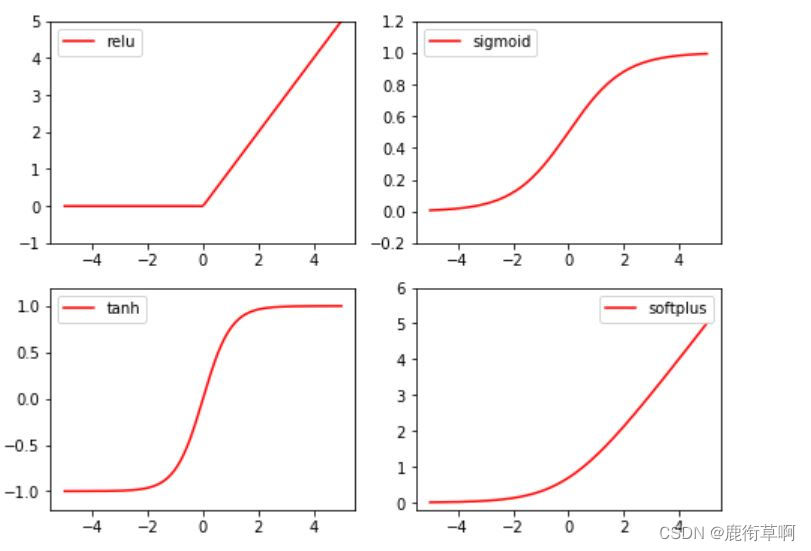
4. 激励函数 (Activation)
常见的激励函数:Relu, Sigmoid, Tanh, Softplus
import torch
import torch.nn.functional as F     # 激励函数都在这
from torch.autograd import Variable

x = torch.linspace(-5, 5, 200)  # x data (tensor), shape=(100, 1)
x = Variable(x)
print(x.shape)

import matplotlib.pyplot as plt

plt.figure(1, figsize=(8, 6))
plt.subplot(221)
plt.plot(x_np, y_relu, c='red', label='relu')
plt.ylim((-1, 5))
plt.legend(loc='best')

plt.subplot(222)
plt.plot(x_np, y_sigmoid, c='red', label='sigmoid')
plt.ylim((-0.2, 1.2))
plt.legend(loc='best')

plt.subplot(223)
plt.plot(x_np, y_tanh, c='red', label='tanh')
plt.ylim((-1.2, 1.2))
plt.legend(loc='best')

plt.subplot(224)
plt.plot(x_np, y_softplus, c='red', label='softplus')
plt.ylim((-0.2, 6))
plt.legend(loc='best')

plt.show()
5. Regression
import torch
import torch.nn.functional as F     # 激励函数都在这
import matplotlib.pyplot as plt
x = torch.unsqueeze(torch.linspace(-1, 1, 100), dim=1)  # x data (tensor), shape=(100, 1)
y = x.pow(2) + 0.2*torch.rand(x.size())                 # noisy y data (tensor), shape=(100, 1)

# 画图
plt.scatter(x.data.numpy(), y.data.numpy())
plt.show()

torch.unsqueeze(input, dim, out=None) 作用:扩展维度 返回一个新的张量,对输入的既定位置插入维度 1 注意: 返回张量与输入张量共享内存,所以改变其中一个的内容会改变另一个
torch.linspace(start, end, steps=100, out=None) 返回一个1维张量,包含在区间start和end上均匀间隔的step个点。输出张量的长度由steps决定。
参数: start (float) - 区间的起始点 end (float) - 区间的终点 steps (int) - 在start和end间生成的样本数 out (Tensor, optional) - 结果张量
torch.rand(*sizes, out=None) → Tensor 返回一个张量,包含了从区间[0,1)的均匀分布中抽取的一组随机数,形状由可变参数sizes 定义。
参数: sizes (int…) – 整数序列,定义了输出形状 out (Tensor, optinal) - 结果张量
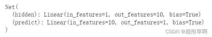
6. 建立神经网络
class Net(torch.nn.Module):  # 继承 torch 的 Module
    def __init__(self, n_feature, n_hidden, n_output):
        super(Net, self).__init__()     # 继承 __init__ 功能
        # 定义每层用什么样的形式
        self.hidden = torch.nn.Linear(n_feature, n_hidden)   # 隐藏层线性输出
        self.predict = torch.nn.Linear(n_hidden, n_output)   # 输出层线性输出

    def forward(self, x):   # 这同时也是 Module 中的 forward 功能
        # 正向传播输入值, 神经网络分析出输出值
        x = F.relu(self.hidden(x))      # 激励函数(隐藏层的线性值)
        x = self.predict(x)             # 输出值
        return x

net = Net(n_feature=1, n_hidden=10, n_output=1)

print(net)
net2 = torch.nn.Sequential(
    torch.nn.Linear(1, 10),
    torch.nn.ReLU(),
    torch.nn.Linear(10, 1)
)
print(net2)

7. 训练网络
# optimizer 是训练的工具
optimizer = torch.optim.SGD(net.parameters(), lr=0.2)  # 传入 net 的所有参数, 学习率
loss_func = torch.nn.MSELoss()      # 预测值和真实值的误差计算公式 (均方差)

epochs = 200

plt.ion()   # 画图
plt.show()

for t in range(epochs):
    prediction = net(x)     # 喂给 net 训练数据 x, 输出预测值

    loss = loss_func(prediction, y)     # 计算两者的误差

    optimizer.zero_grad()   # 清空上一步的残余更新参数值
    loss.backward()         # 误差反向传播, 计算参数更新值
    optimizer.step()        # 将参数更新值施加到 net 的 parameters 上

    #画图
    if t % 5 == 0:
        # plot and show learning process
        plt.cla()
        plt.scatter(x.data.numpy(), y.data.numpy())
        plt.plot(x.data.numpy(), prediction.data.numpy(), 'r-', lw=5)
        plt.text(0.5, 0, 'Loss=%.4f' % loss.data.numpy(), fontdict={
    'size': 20, 'color':  'red'})
        plt.pause(0.1)
边栏推荐
- Strategy mode
- Arduino Serial系列函数 有关print read 的总结
- Deep learning parameter initialization (I) Xavier initialization with code
- 【已解决】Unknown error 1146
- Advanced API (multithreading 02)
- 691. Cube IV
- 高并发内存池
- SecureCRT password to cancel session recording
- The babbage industrial policy forum
- Map interface and method
猜你喜欢

Leetcode 198: 打家劫舍

1. E-commerce tool cefsharp autojs MySQL Alibaba cloud react C RPA automated script, open source log

Le Seigneur des anneaux: l'anneau du pouvoir

你开发数据API最快多长时间?我1分钟就足够了
7.2刷题两个
【开发笔记】基于机智云4G转接板GC211的设备上云APP控制
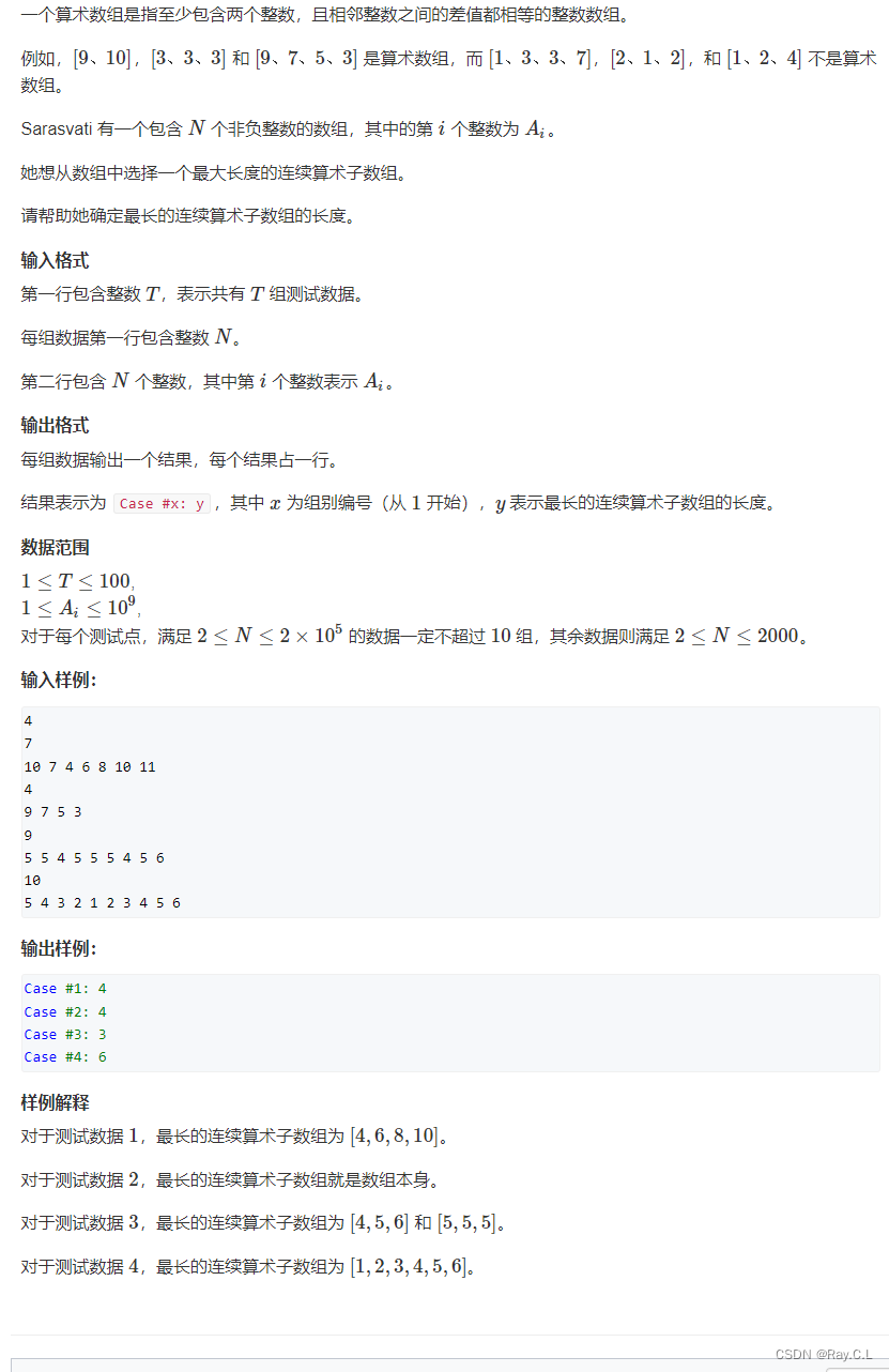
3311. 最长算术
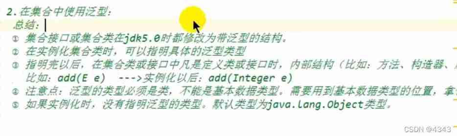
Use of generics

C code production YUV420 planar format file
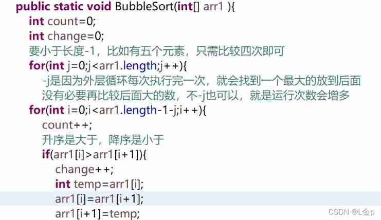
Sorting, dichotomy
随机推荐
Summary of abnormal mechanism of interview
C WinForm framework
Store WordPress media content on 4everland to complete decentralized storage
Arduino Serial系列函数 有关print read 的总结
Jeecg menu path display problem
Beginners use Minio
[set theory] Stirling subset number (Stirling subset number concept | ball model | Stirling subset number recurrence formula | binary relationship refinement relationship of division)
Win 2008 R2 crashed at the final installation stage
[HCAI] learning summary OSI model
Download address collection of various versions of devaexpress
Map interface and method
Realize the reuse of components with different routing parameters and monitor the changes of routing parameters
4279. 笛卡尔树
Final, override, polymorphism, abstraction, interface
gstreamer ffmpeg avdec解码数据流向分析
Introduction of buffer flow
"Moss ma not found" solution
Recursion, Fibonacci sequence
Advanced API (serialization & deserialization)
Advanced API (character stream & net for beginners)