当前位置:网站首页>Deep learning parameter initialization (I) Xavier initialization with code
Deep learning parameter initialization (I) Xavier initialization with code
2022-07-03 07:04:00 【Xiaoshu Xiaoshu】
Catalog
3、 ... and 、 Standard initialization method
Four 、Xavier Initialization assumptions
5、 ... and 、Xavier Simple formula derivation of initialization :
6、 ... and 、Pytorch Realization :
7、 ... and 、 Comparative experiments
1. Histogram of activation value of each layer
2. Gradient of back propagation of each layer ( About the gradient of states ) Distribution of
3. Distribution of parameter gradient in each layer
4. Distribution of weight gradient variance of each layer
One 、 brief introduction
Xavier Initialization is also called Glorot initialization , Because the inventor was Xavier Glorot.Xavier initialization yes Glorot Another initialization method proposed by et al. In order to solve the problem of random initialization , Their idea is to make input and output obey the same distribution as much as possible , In this way, the output value of the activation function in the later layer can be avoided to tend to 0.
Because weights are usually initialized with Gauss or uniform distribution , And there won't be much difference between the two , As long as the variance of the two is the same , So let's say Gaussian and uniform distribution together .
Pytorch There are already implementations in , I'll give you a detailed introduction :
torch.nn.init.xavier_uniform_(tensor: Tensor, gain: float = 1.)
torch.nn.init.xavier_uniform_(tensor: Tensor, gain: float = 1.)
Two 、 Basic knowledge of
1. Variance of uniform distribution :
2. Suppose that random variables X And random variables Y Are independent of each other , Then there are

3. Suppose that random variables X And random variables Y Are independent of each other , And E(X)=E(Y)=0, Then there are

3、 ... and 、 Standard initialization method
When the weight initialization meets the uniform distribution :

Because the formula (1) The variance of : , So the corresponding Gaussian distribution is written :
For a fully connected network , Let's enter X Every dimension of x As a random variable , And suppose E(x)=0,Var(x)=1. Suppose the weight W And the input X Are independent of each other , Then the variance of the hidden layer state is :

It can be seen that the standard initialization method has a very good feature : The mean value of the state of the hidden layer is 0, The variance is constant 1/3, It has nothing to do with the number of layers of the network , This means that for sigmoid For such a function , The independent variable falls within the gradient range .
But because sigmoid Activation values are greater than 0 Of , It will cause the input of the next layer to be unsatisfied E(x)=0. In fact, the standard initialization is only applicable to meet the following Glorot Assumed activation function , such as tanh.
Four 、Xavier Initialization assumptions
At the beginning of the article, we give the necessary conditions for parameter initialization . But these two conditions only ensure that useful information can be learned during the training —— The parameter gradient is not 0( Because the parameter is controlled in the effective area of the active function ). and Glorot Think : Excellent initialization should make the activation value of each layer consistent with the variance of the state gradient in the propagation process . That is to say, we should ensure that the variance of the parameters of each layer of forward propagation is consistent with that of each layer of back propagation :
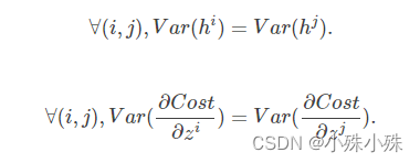
We call these two conditions Glorot Conditions .
combined , Now let's make the following assumptions :
1. The variance of each feature input is the same :Var(x);
2. Activate function symmetry : In this way, it can be assumed that the input mean value of each layer is 0;
3.f′(0)=1
4. At the beginning , The state value falls in the linear region of the activation function :f′(Si(k))≈1.
The last three are all assumptions about activation functions , We call it Glorot The activation function assumes .
5、 ... and 、Xavier The initialization of the Simple formula derivation :
First, the expressions of the gradient of the state and the gradient of the parameter are given :

Let's take the fully connected layer as an example , Expression for :

among ni Indicates the number of inputs .
According to the knowledge of probability and statistics, we have the following variance formula :
Special , When we assume that the input and weight are 0 Mean time ( There is now BN after , This is also easier to meet ), The above formula can be simplified as :

Assume that the input x And weight w Independent homologous distribution , In order to ensure that the input and output variances are consistent , There should be :
For a multi-layer network , The variance of a certain layer can be expressed in the form of accumulation , Is the current number of layers :

Special , Back propagation has a similar form when calculating the gradient :

Sum up , In order to ensure that the variance of each layer is consistent in forward propagation and back propagation , Should satisfy :

however , In practice, the number of inputs and outputs is often not equal , So for balance , We will input and output l The variance of the two layers is taken as the mean , Finally, our weight variance should meet :
therefore Xavier Initialized Gaussian distribution formula :
According to the variance formula of uniform distribution :
And because here |a|=|b|, therefore Xavier The implementation of initialization is the following uniform distribution :
6、 ... and 、Pytorch Realization :
import torch

#  Defining models   Three layer convolution   One layer full connection
class DemoNet(torch.nn.Module):
    def __init__(self):
        super(DemoNet, self).__init__()
        self.conv1 = torch.nn.Conv2d(1, 1, 3)
        print('random init:', self.conv1.weight)
        '''
        xavier  The initialization method obeys uniform distribution  U(−a,a) , Parameters of the distribution  a = gain * sqrt(6/fan_in+fan_out),
         Here's one  gain, The gain is set according to the type of activation function , This initialization method , Also known as  Glorot initialization
        '''
        torch.nn.init.xavier_uniform_(self.conv1.weight, gain=1)
        print('xavier_uniform_:', self.conv1.weight)
        '''
            xavier  The initialization method obeys the normal distribution ,
            mean=0,std = gain * sqrt(2/fan_in + fan_out)
        '''
        torch.nn.init.xavier_uniform_(self.conv1.weight, gain=1)
        print('xavier_uniform_:', self.conv1.weight)


if __name__ == '__main__':
    demoNet = DemoNet()
7、 ... and 、 Comparative experiments
Experimental use tanh Is the activation function
1. Histogram of activation value of each layer
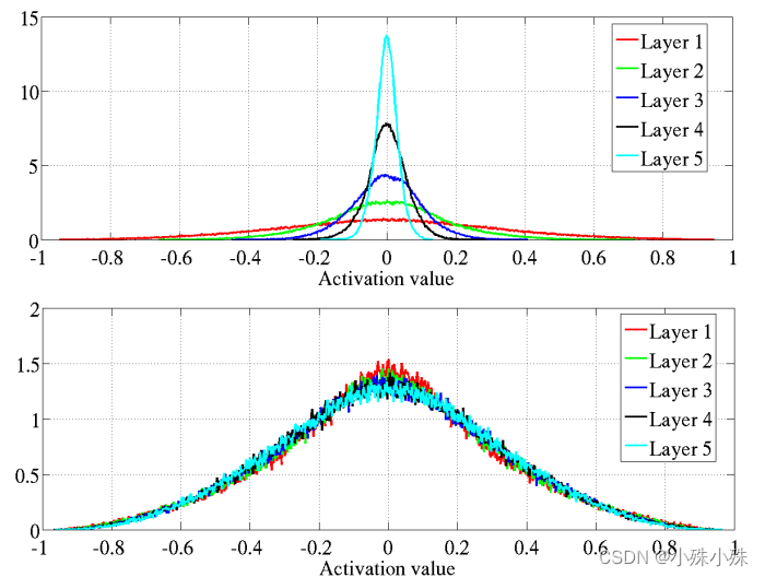
The above figure shows the original initialization , The picture below is Xavier initialization .Xavier The activation values of each layer of the initialized network are relatively consistent , And the values are smaller than the original standard initialization .
2. Gradient of back propagation of each layer ( About the gradient of states ) Distribution of

The above figure shows the original initialization , The picture below is Xavier initialization .Xavier The gradient of each layer of the initialized network is relatively consistent , And the values are smaller than the original standard initialization . The author suspects that different gradients on different layers may lead to morbidity or slow training .
3. Distribution of parameter gradient in each layer
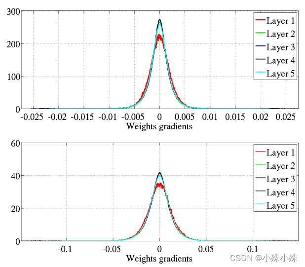
Formula (3) It has been proved that the variance of the parameter gradient of each layer is basically independent of the number of layers . The above figure shows the original initialization , The picture below is Xavier initialization . We find that the standard initialization parameter gradient in the figure below is one order of magnitude smaller .
4. Distribution of weight gradient variance of each layer

The above figure shows the original initialization , The picture below is Xavier initialization .Xavier The variance of initialization weight gradient is consistent .
8、 ... and 、 summary
1.Xavier Initialized Gaussian distribution formula :

2.Xavier Initialized uniform distribution formula :
3.Xavier Initialization is based on the standard initialization method , It takes into account the parameter variance of each layer in forward propagation and shared propagation .
4.Xavier Initial shortcomings : because Xavier The derivation of is based on several assumptions , One of them is that the activation function is linear . This does not apply to ReLU Activation function . The other is the activation value about 0 symmetry , This does not apply to sigmoid Functions and ReLU function . In the use of sigmoid Functions and ReLU Function time , Standard initialization and Xavier Initial activation obtained by initialization 、 The parameter gradient characteristics are the same . The variance of the activation value decreases layer by layer , The variance of the parameter gradient also decreases layer by layer .
边栏推荐
- Golang operation redis: write and read hash type data
- The 10000 hour rule won't make you a master programmer, but at least it's a good starting point
- Advanced API (UDP connection & map set & collection set)
- Journal quotidien des questions (11)
- Search engine Bing Bing advanced search skills
- Resthighlevelclient gets the mapping of an index
- How can I split a string at the first occurrence of “-” (minus sign) into two $vars with PHP?
- Win 10 find the port and close the port
- What are the characteristics and functions of the scientific thinking mode of mechanical view and system view
- Tool class static method calls @autowired injected service
猜你喜欢

10000小時定律不會讓你成為編程大師,但至少是個好的起點
La loi des 10 000 heures ne fait pas de vous un maître de programmation, mais au moins un bon point de départ
Interfaces and related concepts
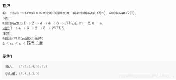
Specified interval inversion in the linked list
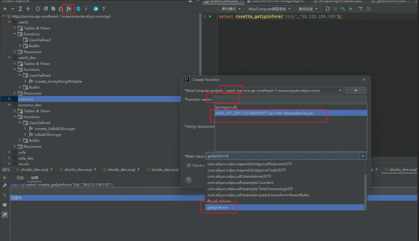
dataworks自定义函数开发环境搭建

Personally design a highly concurrent seckill system
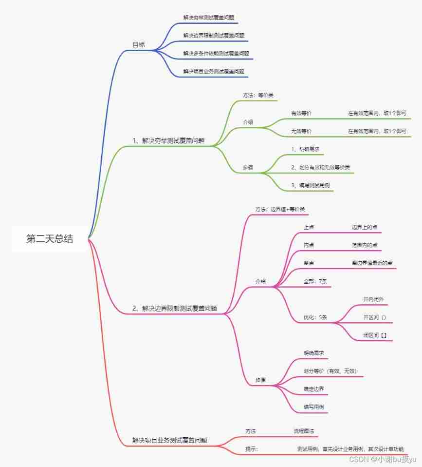
Software testing learning - the next day
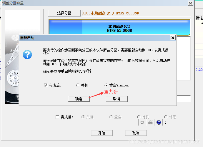
vmware虚拟机C盘扩容

机器学习 | 简单但是能提升模型效果的特征标准化方法(RobustScaler、MinMaxScaler、StandardScaler 比较和解析)

(翻译)异步编程:Async/Await在ASP.NET中的介绍
随机推荐
RestHighLevelClient获取某个索引的mapping
How to specify the execution order for multiple global exception handling classes
Stream stream
golang操作redis:写入、读取hash类型数据
多个全局异常处理类,怎么规定执行顺序
How can the server set up multiple interfaces and install IIS? Tiantian gives you the answer!
机器学习 | 简单但是能提升模型效果的特征标准化方法(RobustScaler、MinMaxScaler、StandardScaler 比较和解析)
JMeter JSON extractor extracts two parameters at the same time
Advanced API (local simulation download file)
In depth analysis of reentrantlock fair lock and unfair lock source code implementation
Resttemplate configuration use
Redis command
What are the characteristics and functions of the scientific thinking mode of mechanical view and system view
Inno Setup 制作安装包
Application scenarios of Catalan number
Advanced APL (realize group chat room)
Troubleshooting of high CPU load but low CPU usage
Class and object summary
How can I split a string at the first occurrence of “-” (minus sign) into two $vars with PHP?
[vscode - vehicle plug-in reports an error] cannot find module 'xxx' or its corresponding type declarations Vetur(2307)