[deep learning]: day 1 of pytorch introduction to project practice: data operation and automatic derivation

【 Deep learning 】:PyTorch: Data manipulation and automatic derivation

• This article is included in 【 Deep learning 】：《PyTorch Introduction to project practice 》 special column , This column mainly records how to use PyTorch Realize deep learning notes , Try to keep updating every week , You are welcome to subscribe ！
• Personal home page ：JoJo Data analysis adventure
• Personal introduction ： I'm reading statistics in my senior year , At present, Baoyan has reached statistical top3 Colleges and universities continue to study for Postgraduates in Statistics
• If it helps you , welcome Focus on 、 give the thumbs-up 、 Collection 、 subscribe special column

Reference material ： This column focuses on bathing God 《 Hands-on deep learning 》 For learning materials , Take notes of your study , Limited ability , If there is a mistake , Welcome to correct . At the same time, Musen uploaded teaching videos and teaching materials , You can go to study .

• video ： Hands-on deep learning
• The teaching material ： Hands-on deep learning

1. Data manipulation

#  Import torch
import torch 
import numpy as np

1.1 Tensor creation

x = torch.arange(12)
y = np.arange(12)

x,y

(tensor([ 0,  1,  2,  3,  4,  5,  6,  7,  8,  9, 10, 11]),
 array([ 0,  1,  2,  3,  4,  5,  6,  7,  8,  9, 10, 11]))

tensor( tensor ) Represents an array of numeric values , There can be multiple dimensions , similar numpy Medium n Dimension group , So many n Some methods of dimension group also have tensor , Now let's test what numpy The method in can be used here . To understand numpy You can read this article ：
Python Data analysis big killer Numpy Detailed explanation

#  Look at shapes 
x.shape

torch.Size([12])

#  Check the quantity and length 
len(x)

12

It can also be used reshape Function to convert an array

x = x.reshape(3,4)
x

tensor([[ 0,  1,  2,  3],
        [ 4,  5,  6,  7],
        [ 8,  9, 10, 11]])

zeros Create all for 0 The elements of

x = torch.zeros(3,4)
x

tensor([[0., 0., 0., 0.],
        [0., 0., 0., 0.],
        [0., 0., 0., 0.]])

ones Create all for 1 The elements of

x = torch.ones(3,4)
x

tensor([[1., 1., 1., 1.],
        [1., 1., 1., 1.],
        [1., 1., 1., 1.]])

eye Create diagonal matrix

l = torch.eye(5)
l

tensor([[1., 0., 0., 0., 0.],
        [0., 1., 0., 0., 0.],
        [0., 0., 1., 0., 0.],
        [0., 0., 0., 1., 0.],
        [0., 0., 0., 0., 1.]])

ones_like Create all shapes that are consistent 1 Element matrix of

x = torch.ones_like(l)
x

tensor([[1., 1., 1., 1., 1.],
        [1., 1., 1., 1., 1.],
        [1., 1., 1., 1., 1.],
        [1., 1., 1., 1., 1.],
        [1., 1., 1., 1., 1.]])

randn Create a random matrix

x =  torch.randn((2,4))
x

tensor([[-0.2102, -1.5580, -1.0650, -0.2689],
        [-0.5349,  0.6057,  0.7164,  0.4334]])

There can be multiple dimensions , As shown below , Create a two-dimensional tensor, among 0 Represents the outer floor ,1 Represents an internal layer

x = torch.tensor([[1,1,1,1],[1,2,3,4],[4,3,2,1]])
x 

tensor([[1, 1, 1, 1],
        [1, 2, 3, 4],
        [4, 3, 2, 1]])

Tensors can also be related to numpy The arrays of are converted to each other , The details are as follows

y = x.numpy()
type(x),type(y)

(torch.Tensor, numpy.ndarray)

1.2 Basic operation

After creating the tensor , We are interested in how to calculate these tensors . Like multidimensional arrays , Tensors can also perform some basic operations , The specific code is as follows

x = torch.tensor([1,2,3,4])
y = torch.tensor([2,3,4,5])
x+y,x-y,x*y,x/y

(tensor([3, 5, 7, 9]),
 tensor([-1, -1, -1, -1]),
 tensor([ 2,  6, 12, 20]),
 tensor([0.5000, 0.6667, 0.7500, 0.8000]))

It can be seen that and numpy Array is the same , It is also an operation on elements . Let's look at the summation operation

x = torch.arange(12).reshape(3,4)
x.sum(dim=0)# Sum up by line 

tensor([12, 15, 18, 21])

y = np.arange(12).reshape((3,4))
y.sum(axis=0)# Sum up by line 

array([12, 15, 18, 21])

As can be seen from the above ,tensor and array Can be operated by row or case , But in torch in , Appoint dim Parameters ,numpy in , Appoint axis Parameters

1.3 Broadcast mechanism

Our previous numpy Broadcast mechanism has been introduced in , When two arrays have different latitudes , You can copy elements appropriately to expand elements of one or two latitudes , So let's see torch Does China also support broadcast mechanism

x = torch.tensor([[1,2,3],[4,5,6]])
y = torch.tensor([1,1,1])
z = x + y
print('x:',x)
print('y:',y)
print('z:',z)

x: tensor([[1, 2, 3],
        [4, 5, 6]])
y: tensor([1, 1, 1])
z: tensor([[2, 3, 4],
        [5, 6, 7]])

Through the above code, we can find ,torch Broadcast mechanism is also supported in , and numpy The use in is basically the same

1.4 Index and slice

Next, let's see how to treat tensor The results were sliced and indexed , Usage and numpy Almost the same

x

tensor([[1, 2, 3],
        [4, 5, 6]])

#  Select the data of the first and second columns 
x[:,[0,1]]

tensor([[1, 2],
        [4, 5]])

2. Automatic differentiation （ Derivation ）

Linear algebra, you can see my numpy article , There is a specific introduction , Let's focus on how to find the derivative .
In deep learning , For many layers of neural networks , Artificial derivation is a very complicated thing , Therefore, it is very important to find the derivative automatically work Things about

Here we assume to be right $y=x^{T}x$ To find the derivative . First, we initialize a x value

x = torch.arange(4.0)
x

tensor([0., 1., 2., 3.])

Now, before we calculate the gradient , You need a place to store the gradient , Like when we're doing some cycles , Need an empty list to store content . Let's see how to use requires_grad_ To store

x.requires_grad_(True)
print(x.grad)# The default is None, Equivalent to an empty list at this time 

None

Let's calculate y

y = torch.dot(x,x)
y

tensor(14., grad_fn=<DotBackward0>)

#  The gradient is calculated by the back propagation function 
y.backward(retain_graph=False)
x.grad

tensor([0., 2., 4., 6.])

Here, by default ,pytorch Will save the gradient , So when we need to recalculate the gradient , The first step is to initialize , Use grad.zero_

x.grad.zero_()
#  Recalculate y=x Gradient of 
y = x.sum()
y.backward()
x.grad

tensor([1., 1., 1., 1.])

Above, we all put y Become a scalar and find the gradient , If y It's not scalar ？ You can put y Convert summation to scalar

x.grad.zero_()
y = x*x
y.sum().backward()
x.grad

tensor([0., 2., 4., 6.])

2.3 Separate differential calculation

Here, God Mu gives such a scene ,y It's about x Function of , and z It's about y and x Function of , Before we get to z seek x Partial derivative time , We hope that y As a constant . This method is very effective in some complex neural network models , Concrete adoption detach() Realization , take u by y The constant

The specific code is as follows ：

x.grad.zero_()# Initialization gradient 
y = x * x#y Yes x Function of 
u = y.detach()# take y Separation treatment 
z = u * x#z Yes x Function of 
z.sum().backward()# Find the gradient through the back propagation function 
x.grad

tensor([0., 1., 4., 9.])

What are the above results ？ According to the law of derivation :
$$\frac{dz}{dx}=u$$
Let's take a look at u How much is the

u

tensor([0., 1., 4., 9.])

2.4 Control flow gradient calculation

One advantage of using automatic differentiation is , When our function is piecewise , It will also automatically calculate the corresponding gradient . Let's look at a case of gradient calculation of linear control flow ：

def f(a):
    if a.sum() > 0:
        b = a
    else:
        b = 100 * a
    return b

First, we define a linear piecewise function , As shown above ：
$$f(a)=\{\begin{array}{ll}a& \text{a.sum()>0}\\ 100\ast a& \text{else}\end{array}$$

Now let's look at how to do automatic derivation

a = torch.randn(12, requires_grad=True)
d = f(a)
d.backward(torch.ones_like(a))
a.grad == d / a

tensor([True, True, True, True, True, True, True, True, True, True, True, True])

Practice and summary

1. Redesign an example of finding the gradient of control flow , Run and analyze the results .

In the case above , Mu Shen gave an example of a linear piecewise function , Suppose it's not linear , Let's assume that a piecewise function is like this
$$f(x)=\{\begin{array}{ll}x& \text{norm(x)>10}\\ x^2& \text{else}\end{array}$$
The specific control flow code is as follows ：

def f(x):
    if x.norm() > 10:
        y = x
    else:
        y = x*x
    return y

x = torch.randn(12,requires_grad=True)
y = f(x)
y.backward(torch.ones_like(x))
x.grad

tensor([ 0.3074, -2.0289,  0.5950,  1.2339, -2.2543,  0.5834, -2.3040, -1.9097,
         0.9255,  1.6837, -1.4464, -0.3131])

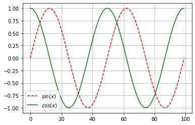
2. Draw differential diagram

send $f(x)=sin(x)$, draw $f(x)$ and $\frac{df(x)}{dx}$ Image , The latter does not use $f^{\prime }(x)=cos(x)$, Here we also need to use matplotlib, If you want to know something, you can read my article ：

import numpy as np
import matplotlib.pyplot as plt
%matplotlib inline

x = torch.linspace(-2*torch.pi, 2*torch.pi, 100)
x.requires_grad_(True)
y = torch.sin(x)
y.sum().backward()
y = torch.detach(y)
plt.plot(y,'r--',label='$sin(x)$')
plt.plot(x.grad,'g',label='$cos(x)$')
plt.legend(loc='best')
plt.grid()

​

​

This is the introduction of this chapter , If it helps you , Please do more thumb up 、 Collection 、 Comment on 、 Focus on supporting ！！