author |Samarendra Chandan Bindu Dash
compile |Flin
source |analyticsvidhya
Introduce
In this paper , We're going to delve into an interesting algorithm , be called “ Seam carving ”. It seems impossible to resize an image without clipping or distorting its contents . We will gradually build , Starting from scratch to achieve seam carving algorithm , And look at some interesting mathematical principles behind it .
The knowledge of calculus will be helpful to the follow-up study , But not necessarily . Let's start .
( This article is inspired by grant of MIT · Sanderson's speech .)
problem
Let's take a look at this picture .

El Salvador · Dali (Salvador Dali) The finished painting is named “ The eternity of memory ”. We are more interested in the content of painting , Not its artistic value . We want to adjust the size of the picture by reducing its width . Two effective processes we can think of are cutting pictures or compressing width .
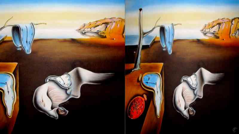
however , As we can see , Clipping removes many objects , Squeezing can distort the image . We want both , That is, reduce the width without clipping any objects or distorting them .
We can see , Apart from the object , There's a lot of blank space in the picture . The task we're going to do here is to somehow delete the blank areas between objects , In order to preserve the interesting parts of the image , At the same time, discard unnecessary space .
It's really a tricky issue , It's easy to get lost . therefore , Break down the problem into smaller ones , The easier part to manage is always a good idea . We can divide the problem into two parts .
- Identify interesting parts of the picture ( Namely object ).
- The logo can be removed without distorting the pixel path of the image .
Identify objects
Before proceeding , We need to convert images to grayscale images . This will be helpful for us to do later . This is a will RGB A simple formula for converting pixels to grayscale values

def rgbToGrey(arr):
    greyVal = np.dot(arr[...,:3], [0.2989, 0.5870, 0.1140])
    return np.round(greyVal).astype(np.int32)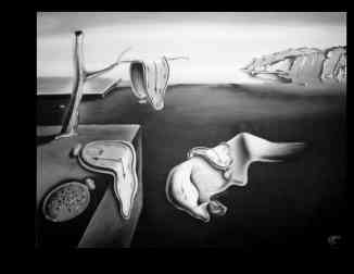
In order to identify objects , We can develop strategies . What if we can identify all the edges in the picture in some way ? then , We can ask the seam carving algorithm to adopt pixel path without passing through the edge , therefore , By extending the , It doesn't touch any area enclosed by the edges .
however , How do we recognize edges ? One observation we can see is , Whenever the color between two adjacent pixels changes dramatically , Most likely, it's the edge of the object . We can rationalize this immediate color change , As the beginning of a new object starting from that pixel .
The next problem we have to solve is how to recognize the sharp changes in pixel values . Now? , Let's consider a simple case , That's a row of pixels . Suppose we represent this array of values as x.

We can take pixels x [i + 1],x [i] The difference between . It shows how much the current pixel has changed from the right . Or we can take x [i] and x [i-1] The difference between the , This will change on the left side . To show the total change , We may have to take the average of the two , obtain

Anyone familiar with calculus can quickly identify this expression as a definition of derivative . We need to calculate x A sharp change in value , So we're calculating its derivative . If we define a filter [ -0.5,0,0.5 ], And then use arrays [x[i-1],x[i],x[i+1] Multiply by its elements , And then take it and , It will get x[i] The derivative of .
Because our picture is 2D Of , So we need to 2D filter . I won't elaborate on , But our filter's 2D The version looks like this ,

When our filter computes along x The derivative of each pixel of the axis , It will give the vertical edge . Again , If we go along y The axis computes the derivative , It will have a horizontal edge . The filter is as follows .( When used with transposition x The filters on the shaft are the same .)

These filters are also known as Sobel filter .
therefore , We have two filters , Need to spread in the picture . For each pixel , use (3X3) A submatrix is multiplied by its elements , And then take it and . This operation is called convolution .
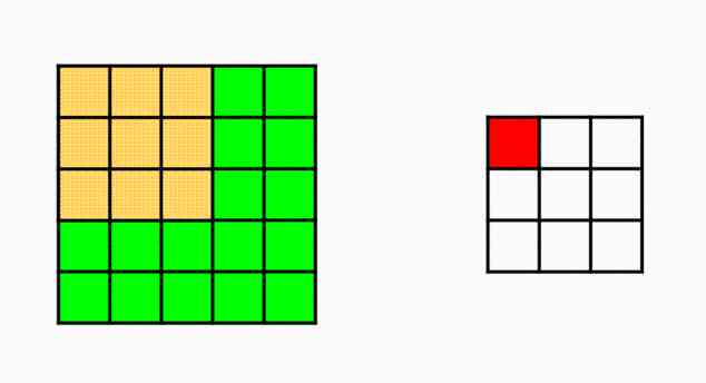
Convolution :
The math , That's how convolution works ,

Let's see how we multiply two functions point by point , And then we integrate it . Numerically , This will correspond to what we have done before , That is, the filter is multiplied by the image element by element , And then sum it up .
Be careful , about k function , How it is written as k(t-τ). Because convolution requires flipping one of the signals . You can intuitively imagine it like this : Two trains collide with each other in a straight horizontal track ( Don't worry about , Because they're superimposed , Nothing will happen to the train ). therefore , The locomotives will face each other . Now? , Suppose you're scanning the orbit from left to right . then , For the left train , You're going to scan from the tail to the head .
Again , The computer needs to go from the lower right corner (2,2) Corner to top left (0,0) Instead of reading the filter from the top left to the bottom right . therefore , Actually Sobel The filter looks like this ,

Before convolution , Let's go ahead 180 Degree of rotation .

We can continue to write a simple implementation to convolute operations . like this :
def naiveConvolve(img,ker):

    res = np.zeros(img.shape)
    r,c = img.shape
    rK,cK = ker.shape
    halfHeight,halfWidth = rK//2,cK//2

    ker = np.rot90(ker,2)
    img = np.pad(img,((1,1),(1,1)),mode='constant')

    for i in range(1,r+1):
        for j in range(1,c+1):
            res[i-1,j-1] = np.sum(np.multiply(ker,img[i-halfHeight:i+halfHeight+1,j-halfWidth:j+halfWidth+1]))

    return res
It will work well , But it will take a lot of time to implement , Because it's going to be close to 9 r c Multiplication and addition operations to get the result . But we can use more concepts in mathematics cleverly to reduce time complexity .
Fast convolution :
Convolution has interesting properties . Convolution in time domain corresponds to multiplication in frequency domain . namely

, among F(w) Represents a function in the frequency domain .
We know that Fourier transform transforms the signal in time domain into its frequency domain . therefore , What we can do is calculate the Fourier transform of the image and the filter , Multiply them by , Then inverse Fourier transform is performed to obtain the convolution result .
For this we can use NumPy library .
def fastConvolve(img,ker):
    imgF = np.fft.rfft2(img)
    kerF = np.fft.rfft2(ker,img.shape)
    return np.fft.irfft2(imgF*kerF)
( Be careful : In some cases , The value obtained may be slightly different from the simple method , because fastConvolve Function will calculate circular convolution . But actually , We can easily use fast convolution , You don't have to worry about these small differences in values .)
cool ! Now? , We have an effective way to calculate horizontal and vertical edges , namely x and y component . therefore , Use

def getEdge(greyImg):

    sX = np.array([[0.25,0.5,0.25],
                   [0,0,0],
                   [-0.25,-0.5,-0.25]])
    sY = np.array([[0.25,0,-0.25],
                   [0.5,0,-0.5],
                   [0.25,0,-0.25]])

    #edgeH = naiveConvolve(greyImg,sX)
    #edgeV = naiveConvolve(greyImg,sY)
    edgeH = fastConvolve(greyImg,sX)
    edgeV = fastConvolve(greyImg,sY)

    return np.sqrt(np.square(edgeH) + np.square(edgeV))
Identify pixel paths :
For continuous paths , We can define a rule , That is, each pixel is only connected to the 3 Nearest pixels . This will allow pixels to have a continuous path from top to bottom . therefore , Our subproblem becomes the basic pathfinding problem , We have to keep costs to a minimum .
Because the edge has a higher amplitude , If we continue to remove pixel paths at the lowest cost , It will avoid the appearance of edges .
Let's define a function “ cost”, This function takes a pixel and calculates the minimum cost pixel path from there to the end of the picture . We have the following observations ,
- At the bottom line ( namely i = r-1)

- For any intermediate pixel ,

Code :
def findCostArr(edgeImg):
    r,c = edgeImg.shape
    cost = np.zeros(edgeImg.shape)
    cost[r-1,:] = edgeImg[r-1,:]

    for i in range(r-2,-1,-1):

        for j in range(c):
            c1,c2 = max(j-1,0),min(c,j+2)
            cost[i][j] = edgeImg[i][j] + cost[i+1,c1:c2].min()

    return cost
mapping :

We can see the triangle in the picture . They represent points that don't return , in other words , If you get to that pixel , There's no path that doesn't go through the edge to the bottom . And that's exactly what we're trying to avoid .
It is easy to find pixel path from cost matrix by greedy algorithm . Find the lowest cost pixel in the top row , Then move down , Choose the lowest cost pixel of all the pixels connected to it .
def findSeam(cost):

    r,c = cost.shape

    path = []
    j = cost[0].argmin()
    path.append(j)

    for i in range(r-1):
        c1,c2 = max(j-1,0),min(c,j+2)
        j = max(j-1,0)+cost[i+1,c1:c2].argmin()
        path.append(j)

    return path
To remove the seam defined by the path , We just need to traverse each row and delete the columns mentioned in the path array .
def removeSeam(img,path):
    r,c,_ = img.shape
    newImg = np.zeros((r,c,3))
    for i,j in enumerate(path):
        newImg[i,0:j,:] = img[i,0:j,:]
        newImg[i,j:c-1,:] = img[i,j+1:c,:]
    return newImg[:,:-1,:].astype(np.int32)
ad locum , I've calculated in advance 100 Seam carving operations .
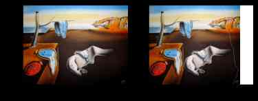

We can see how the objects in the painting approach each other . We have successfully reduced the size of the image using seam cutting algorithm , And it doesn't deform anything . I've attached a link to the full code . Interested readers can take a look here .
in general , Seam carving is an interesting algorithm . It has some warnings , Because if the image provided has too much detail or too many edges , It will fail .
It is always interesting to use this algorithm to modify different pictures to see the final results . If you have any questions or suggestions , Please leave me a message .
Thanks for reading !
Link to the original text :https://www.analyticsvidhya.c...
Welcome to join us AI Blog station :
http://panchuang.net/
sklearn Machine learning Chinese official documents :
http://sklearn123.com/
Welcome to pay attention to pan Chuang blog resource summary station :
http://docs.panchuang.net/


