当前位置:网站首页>Optimal transport Series 1
Optimal transport Series 1
2022-07-01 02:33:00 【Daft shiner】
Whereas Optimal Transport stay Machine Learning Widespread use in the field , I want to study it carefully Optimal Transport, There's a lot of information online , But because the author is stupid , It took me a long time to find the easy to understand materials . This blog aims to describe clearly in the simplest way Optimal transport, Due to limited mathematical ability , If there is any mistake, I hope you can correct it in time .
List of articles
Prior Knowledge

L1 Distance: d L 1 ( ρ 1 , ρ 2 ) = ∫ − ∞ + ∞ ∣ ρ 1 ( x ) − ρ 2 ( x ) ∣ d x d_{L_1}(\rho_1,\rho_2)=\int_{-\infty}^{+\infty}|\rho_1(x)-\rho_2(x)|dx dL1(ρ1,ρ2)=∫−∞+∞∣ρ1(x)−ρ2(x)∣dx
KL divergence: d K L ( ρ 1 ∣ ∣ ρ 2 ) = ∫ − ∞ + ∞ ρ 1 ( x ) l o g ρ 1 ( x ) ρ 2 ( x ) d x d_{KL}(\rho_1||\rho_2)=\int_{-\infty}^{+\infty}\rho_1(x)log\frac{\rho_1(x)}{\rho_2(x)}dx dKL(ρ1∣∣ρ2)=∫−∞+∞ρ1(x)logρ2(x)ρ1(x)dx
If you want to measure the above figure ( From references 1) in ρ 1 \rho_1 ρ1 To ρ 2 \rho_2 ρ2 The distance and ρ 1 \rho_1 ρ1 To ρ 3 \rho_3 ρ3 Distance of , Can be found using L1 Distance and KL divergence All fail , All the results are the same .
Be careful : by the way L1 Distance Come on , The same distance is easy to understand , Because it calculates the area of two distributions . And for KL divergence Come on , First of all, it should be noted that it is not a distance measure ,Because it is not symmetric: the KL from ρ 1 ( x ) \rho_1(x) ρ1(x) to ρ 2 ( x ) \rho_2(x) ρ2(x) is generally not the same as the KL from ρ 1 ( x ) \rho_1(x) ρ1(x) to ρ 2 ( x ) \rho_2(x) ρ2(x). Furthermore, it need not satisfy triangular inequality. We will Kullback-Leibler Divergence Change the form to get d K L ( ρ 1 ∣ ∣ ρ 2 ) = ∫ − ∞ + ∞ ρ 1 ( x ) l o g ( ρ 1 ( x ) ) − ρ 1 ( x ) l o g ( ρ 2 ( x ) ) d x d_{KL}(\rho_1||\rho_2)=\int_{-\infty}^{+\infty}\rho_1(x)log(\rho_1(x))-\rho_1(x)log(\rho_2(x))dx dKL(ρ1∣∣ρ2)=∫−∞+∞ρ1(x)log(ρ1(x))−ρ1(x)log(ρ2(x))dx And then put ρ 1 ( x ) l o g ( ρ 1 ( x ) ) \rho_1(x)log(\rho_1(x)) ρ1(x)log(ρ1(x)) and ρ 1 ( x ) l o g ( ρ 2 ( x ) ) \rho_1(x)log(\rho_2(x)) ρ1(x)log(ρ2(x)) Consider two new distributions , Then it is also transformed into the area relationship , Because the former one is the same , Therefore, it mainly depends on the difference of the latter item . For better understanding , Author use python Write a simple demo: Be careful , Here I found a big problem !!!
import math
import numpy as np
import matplotlib.pyplot as plt


def guassian(u, sig):
    #  mean value μ,  Standard deviation δ
    x = np.linspace(-30, 30, 1000000)   #  Domain of definition
    y = np.exp(-(x - u) ** 2 / (2 * sig ** 2)) / (math.sqrt(2*math.pi)*sig) #  Define curve function
    return x, y

x1, y1 = guassian(u=0, sig=math.sqrt(1))
x2, y2 = guassian(u=1, sig=math.sqrt(1))
x3, y3 = guassian(u=2, sig=math.sqrt(1))
plt.plot(x1,y1)
plt.plot(x2,y2)
plt.plot(x3,y3)

z1 = y1 * np.log2(y1) - y1 * np.log2(y2)
z2 = y1 * np.log2(y1) - y1 * np.log2(y3)
# plt.plot(x1, z1)
# plt.plot(x1, z2)
print(np.sum(z1))
print(np.sum(z2))
It is found through experiments that , The results of the experiment were quite different from what was expected , I use KL divergence Calculation ρ 1 \rho_1 ρ1 To ρ 2 \rho_2 ρ2 The distance and ρ 1 \rho_1 ρ1 To ρ 3 \rho_3 ρ3 The distance is not the same , Difference is very big !!!
I visualized the distribution curve of the latter term , Found it completely different , And the value after integration is completely different .( Here I take into account the effect that continuity becomes discreteness , So it was adjusted x Coordinate range and number of points drawn , Do not have what difference ) Later, it was found that , It seems that the curve given in the article is not a Gaussian curve , I feel a little misled , So I changed an example to calculate , Although it is a discrete distribution , But it can still directly reflect the problem (PS, In fact, I'm curious about why Gaussian distribution can't be used , Does anyone know why ):
It can be found that for the above distribution ,L1 Distance and KL divergence All failed .
Optimal Transport
Last section L1 Distance and KL divergence The problem is , This section describes in detail Optimal Transport, First define the problem .Optimal Transport The core of is how to find an optimal transformation to transform one distribution into another , And to minimize the conversion loss .( Be careful : The distribution here can be continuous or discrete ) Here we use the ρ 1 \rho_1 ρ1 and ρ 2 \rho_2 ρ2 give an example :
For ease of understanding , We can ρ 1 \rho_1 ρ1 and ρ 2 \rho_2 ρ2 Imagine a pile of sand , that Optimal Transport The question becomes how to make ρ 1 \rho_1 ρ1 The shape of the sand piled up ρ 2 \rho_2 ρ2 The appearance of , And do the least work . π ( x , y ) \pi(x,y) π(x,y) For from x How much quality of sand is moved to the location y Location , So clearly ρ 1 ( x ) \rho_1(x) ρ1(x) Express x How much quality of sand is there in the location ( In plain English x Height of the position curve ). So the problem can be expressed by the following formula :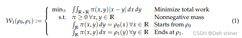
The objective function is to minimize the work done by handling , Because the mass of sand transported should be greater than or equal to 0, So the first constraint is easy to understand , As for articles 2 and 3 , Is to satisfy its initial and final distribution .This amount of work is known as the 1-Wasserstein distance in optimal transport. Next, we generalize it to p-Wasserstein distance:
It is also easy to understand , Only the distance of transportation has changed . After the problem is defined , So how can we get this π ( x , y ) \pi(x,y) π(x,y) Well ?
Discrete Problems in One Dimension

For one-dimensional problems, there are the above two cases :D2D,D2C. about D2D The data of , We first relax the original distribution function ρ ( x ) \rho(x) ρ(x) To μ 0 , μ 1 ∈ P r o b ( R ) \mu_0,\mu_1 \in Prob(\mathbb{R}) μ0,μ1∈Prob(R),Define the Dirac δ \delta δ-measure centered at x ∈ R x \in \mathbb{R} x∈R via (:= In mathematics it is defined as )
δ x ( S ) : = { 1 , i f x ∈ S 0 , O t h e r w i s e . \delta_x(S):= \begin{cases} 1, &if\ x\ \in\ S\\ 0, &Otherwise. \end{cases} δx(S):={ 1,0,if x ∈ SOtherwise. here μ 0 , μ 1 \mu_0,\mu_1 μ0,μ1 Respectively :
among ∑ i a 0 i = ∑ i a 1 i = 1 \sum_ia_{0i}=\sum_ia_{1i}=1 ∑ia0i=∑ia1i=1, a 0 i , a 1 i ≥ 0 a_{0i},a_{1i} \ge 0 a0i,a1i≥0. I think it's S S S yes [ x 01 , x 02 , ⋯ , x 0 k 0 ] [x_{01}, x_{02}, \cdots, x_{0k_0}] [x01,x02,⋯,x0k0] Subset . At this time, the calculation of the problem is :
The same way as the above explanation , T i j T_{ij} Tij From x 0 i x_{0i} x0i Transport to x 1 j x_{1j} x1j The quality of the . ∣ x 0 i − x 1 j ∣ p |x_{0i}-x_{1j}|^p ∣x0i−x1j∣p It's from x 0 i x_{0i} x0i Transport to x 1 j x_{1j} x1j Distance of . T i j T_{ij} Tij The transportation mass shall be greater than or equal to 0, x 0 i x_{0i} x0i and x 1 j x_{1j} x1j The mass at the point must satisfy the conservation condition . requirement T i j T_{ij} Tij, This is a finite element linear programming , Many classical algorithms can be used to solve , for example simplex or interior point methods. And for D2C The situation of , Each discrete μ 0 \mu_0 μ0 Are mapped to a continuous interval μ 1 \mu_1 μ1, As shown in the figure below :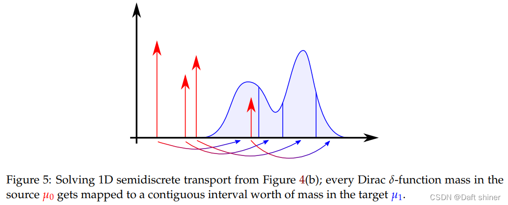
Conclusion
This section focuses on Optimal Transport Two forms of (D2C,D2D), The next section will cover more general In the form of .
References
[1] Optimal Transport on Discrete Domains
[2] Kullback-Leibler Divergence
[3] Optimal Transport and Wasserstein Distance
边栏推荐
- 在unity中使用jieba分词的方法
- Windows quick add boot entry
- Sampling Area Lights
- The latest wechat iPad protocol code obtains official account authorization, etc
- (总结一)Halcon基础之寻找目标特征+转正
- Zero foundation self-study SQL course | window function
- @ConfigurationProperties和@Value的区别
- Pulsar的Proxy支持和SNI路由
- Pytorch —— 基礎指北_貳 高中生都能看懂的[反向傳播和梯度下降]
- Pulsar 主题压缩
猜你喜欢
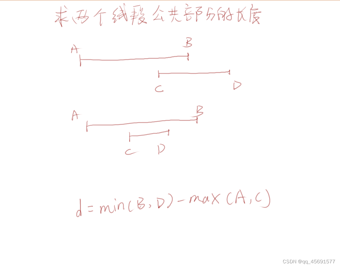
Find the length of the common part of two line segments

Comment réaliser la liaison entre la serrure intelligente et la lampe, la scène du moteur de rideau intelligent dans le timing intelligent?
![[2022] Jiangxi postgraduate mathematical modeling scheme and code](/img/f4/86b0dc2bd49c3a54c1e0538b31d458.png)
[2022] Jiangxi postgraduate mathematical modeling scheme and code

项目管理是什么?

The mobile edge browser cannot open the third-party application

CentOS installs multiple versions of PHP and switches

RestCloud ETL实践之无标识位实现增量数据同步

halcon变量窗口的图像变量不显示,重启软件和电脑都没用

SWT/ANR问题--Binder Stuck

Small program cloud development -- wechat official account article collection
随机推荐
在国内如何买港股的股?用什么平台安全一些?
ANR问题的分析与解决思路
视觉特效,图片转成漫画功能
AI 边缘计算平台 - BeagleBone AI 64 简介
十大劵商如何开户?还有,在线开户安全么?
鼠标悬停效果四
Calculate special bonus
SWT / anr problem - storagemanagerservice stuck
Detailed data governance knowledge system
Is there any discount for opening an account now? In addition, is it safe to open a mobile account?
SWT / anr problem - binder stuck
RestCloud ETL WebService数据同步到本地
鼠标悬停效果十
Contrastive learning of Class-agnostic Activation Map for Weakly Supervised Object Localization and
SWT/ANR问题--Native方法执行时间过长导致SWT
Pulsar geo replication/ disaster recovery / regional replication
@ConfigurationProperties和@Value的区别
鼠标悬停效果七
Alphabet-Rearrange-Inator 3000(字典树自定义排序)
联想X86服务器重启管理控制器(XClarity Controller)或TSM的方法