Pytroch Learning Notes 6: NN network layer convolution layer

Through the previous two sections , You already know how to build a network model and how to build a very important class nn.Module And model containers Containers. There are two basic steps to build a network model ： Create submodules and splice submodules . The established sub module includes convolution layer 、 Pooling layer 、 Activation layer, full connection layer, etc . So this section starts with the sub module .

One 、 Convolution and convolution

Convolution operation ： Convolution kernel in the input signal （ Images ） Slide up , Multiply and add at the corresponding position ;
Convolution layer ： Also known as filter , filter , It can be thought of as a pattern , A certain characteristic .

The process of convolution is similar to using a template to look for areas similar to it in an image , The more similar to the convolution pattern , The higher the activation value , So as to achieve feature extraction .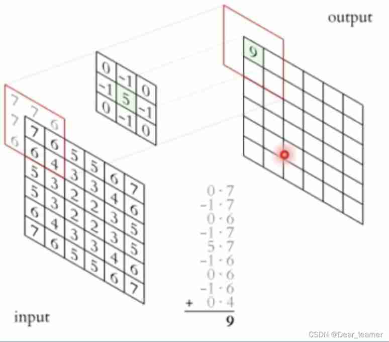

1、1d 2d 3d Convolution scheme

In general , The sliding of convolution kernel on several dimensions is called several dimensional convolution .
One dimensional convolution diagram

Two dimensional convolution diagram

Three dimensional convolution diagram

Two 、 Basic properties of convolution

Convolution kernel (Kernel)： Receptive field of convolution operation , Intuitive understanding is a filter matrix , The commonly used convolution kernel size is 3×3、5×5 etc. ;
step （Stride）： The pixels moved in each step when the convolution kernel traverses the feature map , If the step size is 1 Then every time you move 1 Pixel , In steps of 2 Then every time you move 2 Pixel （ That is, skip 1 Pixel ）, And so on ;
fill （Padding）： How to deal with the boundary of characteristic graph , There are generally two kinds of , One is not to fill the boundary completely , Convolution is performed only on input pixels , This will make the size of the output feature map smaller than the size of the input feature map ; The other is to fill outside the boundary （ Generally filled with 0）, Then perform the convolution operation , In this way, the size of the output feature map can be consistent with the size of the input feature map ;
passageway （Channel）： Number of channels in convolution layer （ The layer number ）.
The following figure shows a convolution kernel （kernel） by 3×3、 step （stride） by 1、 fill （padding） by 1 Two dimensional convolution of ：

3、 ... and 、 Calculation process of convolution

The calculation of convolution is very simple , When the convolution kernel is scanned on the input image , Multiply the convolution kernel one by one with the value of the corresponding position in the input image , Finally, sum up , The convolution result of this position is obtained . Moving convolution kernel , The convolution result of each position can be calculated . Here's the picture ：

Four 、 Various types of convolution

1、 Standard convolution

（1） Two dimensional convolution （ Single channel convolution ）

It has been shown in the diagram above , Represents the convolution of only one channel . The following figure shows a convolution kernel （kernel） by 3×3、 step （stride） by 1、 fill （padding） by 0 Convolution of ：

（2） Two dimensional convolution （ Multichannel convolution ）

Convolution with multiple channels , For example, when processing color images , Respectively for R, G, B this 3 Layer processing 3 Channel convolution , Here's the picture ：

Then the convolution results of the three channels are combined （ Generally, elements are added ）, Get the result of convolution , Here's the picture ：

（3） Three dimensional convolution

Convolution has three dimensions （ Height 、 Width 、 passageway ）, Follow the... Of the input image 3 Slide in two directions , Finally, output the three-dimensional results , Here's the picture ：

（4）1x1 Convolution （1 x 1 Convolution）

When the convolution kernel size is 1x1 Convolution of time , That is, the convolution kernel becomes just one number . Here's the picture ：

As can be seen from the above figure ,1x1 The function of convolution is to effectively reduce the dimension , Reduce computational complexity .1x1 Convolution in GoogLeNet It is widely used in network structure .

2、 deconvolution （ Transposition convolution ）

Convolution is to extract features from the input image （ The size may become smaller ）, The so-called “ deconvolution ” Is to do the opposite . But here it is “ deconvolution ” Not serious , Because it will not be completely restored to the same as the input image , Generally, the restored size is consistent with the input image , It is mainly used for upward sampling . From a mathematical point of view ,“ deconvolution ” So the convolution kernel is transformed into a sparse matrix and transposed , therefore , Also known as “ Transposition convolution ”
Here's the picture , stay 2x2 The step size applied to the input image of is 1、 Full boundary 0 Filled with 3x3 Convolution kernel , Perform transpose convolution （ deconvolution ） Calculation , The output image size after up sampling is 4x4

nn.ConvTranspose2d: Transpose convolution to realize up sampling

The parameters are similar to those of convolution operation .
Size calculation of transpose convolution

3、 Cavity convolution （ Expansion convolution ）

To enlarge the receptive field , Insert a space between the elements in the convolution kernel to “ inflation ” kernel , formation “ Cavity convolution ”（ Or expansion convolution ）, And the expansion rate parameter L Indicates that you want to expand the scope of the kernel , That is, insert... Between kernel elements L-1 A space . When L=1 when , No space is inserted between kernel elements , Change to standard convolution .
The following figure shows the expansion rate L=2 The void convolution of ：

Hole convolution can be understood as a convolution kernel with holes , Commonly used in image segmentation tasks , The main function is to improve the receptive field . That is, a parameter of the output image , You can see a larger area in the front image .

4、 Separable convolution

（1） Space separable convolution

Spatially separable convolution is a function of Convolution kernel It is decomposed into two independent cores to operate separately . One 3x3 The convolution kernel decomposition of is shown in the figure below ：

The convolution calculation process after decomposition is shown in the following figure , First use 3x1 The convolution kernel of is used for transverse scanning calculation , Reuse 1x3 Convolution kernel for longitudinal scanning calculation , Finally, we get the result . The computation of separable convolution is less than that of standard convolution .

（2） Depth separates the convolution

Depth separable convolution consists of two steps ： Deep convolution and 1x1 Convolution .
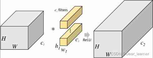
First , Apply depth convolution on the input layer . Here's the picture , Use 3 Convolution kernels , respectively, For input layer 3 Convolution calculation of two channels , Then stack them together .

Reuse 1x1 Convolution of （3 Channels ） Calculate , Only 1 The result of two channels

Repeated many times 1x1 Convolution operation of （ The picture below shows 128 Time ）, Finally, we will get a convolution result of depth .

The whole process is as follows ：


chart a Represents standard convolution , Assume that the dimension of the input characteristic diagram is Df×Df×M, The size of the convolution kernel is Dk×Dk×M, The size of the output feature map is Df×Df×N, The parameter quantity of standard convolution layer is Dk×Dk×M×N.

chart b Represents depth convolution , chart c Represents fractional convolution , The combination of the two is deep separable convolution , Deep convolution is responsible for filtering , Size is Dk×Dk×1, common M individual , Act on each channel of input ; Point by point convolution is responsible for transforming the channel , Size is 1×1×M, common N individual , Acting on the output feature map of depth convolution .

The parameter quantity of depth convolution is Dk×Dk×1×M, The parameter quantity of pointwise convolution is 1×1×M×N, So the parameter quantity of deep separable convolution is the standard convolution parameter quantity ratio is ：

5、 Flat convolution （Flattened convolutions）

Flat convolution is to split the standard convolution kernel into 3 individual 1x1 Convolution kernel , Then convolution calculation is performed on the input layer respectively . This way, , Follow the one in front “ Space separable convolution ” similar , Here's the picture ：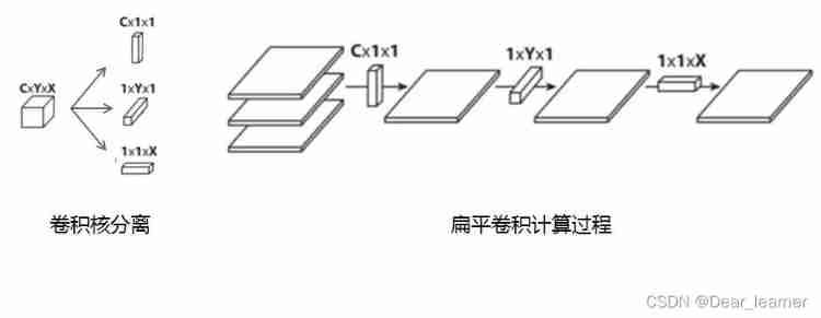

6、 Grouping convolution （Grouped Convolution）

2012 year ,AlexNet The first concept put forward in the paper , At that time, it was mainly to solve GPU The problem of insufficient memory , Put the volume integral group back into two GPU Parallel execution .
In group convolution , Convolution kernels are divided into different groups , Each group is responsible for convolution calculation of the corresponding input layer , Finally, merge . Here's the picture , The convolution kernel is divided into two groups , The convolution group of the first half is responsible for processing the input layer of the first half , The convolution group of the second half is responsible for processing the input layer of the second half , Finally, combine the results .

The first picture is the standard convolution operation , If the dimension of the input characteristic drawing is H×W×c1, The size of the convolution kernel is h1×w1×c1, The size of the output feature map is H×W×c2, Then the parameter quantity of the standard convolution layer is h1×w1×c1×c2.

The second picture represents the block convolution operation , The input characteristic graph is divided into... According to the number of channels g Group , Then the size of each group of characteristic drawings is H×W×（c1/g）, The size of the corresponding convolution kernel is h1×w1×（c1/g）, The size of the feature map output by each group is H×W×（c2/g）, take g Group result stitching （concat）, The size of the final output feature map is H×W×c2, At this time, the parameter quantity of the group convolution layer is ：
h1×w1×（c1/g）×（c2/g）×g=h1×w1×c1×c2×（1/g）

It can be seen that the parameter quantity of the block convolution is that of the standard convolution layer （1/g）

7、 Mix wash group convolution （Shuffled Grouped Convolution）

In group convolution , After the convolution kernel is divided into several groups , The convolution results of the input layer are still combined in the original order , This hinders the flow of feature information between channel groups during training , It also weakens the feature representation . And shuffle packet convolution , That is to mix and cross the calculation results after grouping convolution and output them .
Here's the picture , Group convolution at the first layer （GConv1） After calculation , The obtained feature map shall be disassembled first , Remix crossover , Form a new result input to the layer 2 packet convolution （GConv2） in ：

5、 ... and 、nn.Conv2d Realize two-dimensional convolution

function ： Carry out two-dimensional convolution for multiple two-dimensional plane signals
main parameter ：

• in_channels: Enter the number of channels
• out_channels: Number of output channels , It is equivalent to the number of convolution kernels
• kernel_size: Convolution kernel size , This represents the size of the convolution kernel
• stride: step , When the convolution kernel slips , Slide a few pixels at a time
• padding: Fill in the number of , Usually used to keep a size match between the input and output images ,
• dilation: Hole convolution size
• groups: Group convolution settings , Packet convolution is often used for lightweight models
• bias： bias

Size calculation ：

Let's take a look at how convolution kernel extracts features

set_seed(3)  #  Set random seeds , Change the initialization of random weight 

# ================================= load img ==================================
path_img = os.path.join(os.path.dirname(os.path.abspath(__file__)), "lena.png")
img = Image.open(path_img).convert('RGB')  # 0~255

# convert to tensor
img_transform = transforms.Compose([transforms.ToTensor()])
img_tensor = img_transform(img)
img_tensor.unsqueeze_(dim=0)    # C*H*W to B*C*H*W

# ================================= create convolution layer ==================================

# ================ 2d
flag = 1
# flag = 0
if flag:
    conv_layer = nn.Conv2d(3, 1, 3)   # input:(i, o, size) weights:(o, i , h, w)
    nn.init.xavier_normal_(conv_layer.weight.data)

    # calculation
    img_conv = conv_layer(img_tensor)
# ================================= visualization ==================================
print(" Size before convolution :{}\n The size after convolution :{}".format(img_tensor.shape, img_conv.shape))
img_conv = transform_invert(img_conv[0, 0:1, ...], img_transform)
img_raw = transform_invert(img_tensor.squeeze(), img_transform)
plt.subplot(122).imshow(img_conv, cmap='gray')
plt.subplot(121).imshow(img_raw)
plt.show()

Output results ：

On the left is the original picture , On the right is the image after two-dimensional convolution , It can be seen that it is bright in bright colors . Change the setting of random seed , To change the random initialization value of the weight , You can see the image after convolution with different convolution weights , as follows ：

By setting different random seeds , It can be seen that convolution kernels with different weights represent different patterns , Focus on different features on the image , Therefore, the image features are extracted by setting multiple convolution check , You can get different characteristics .

In addition, the size of the image after convolution ：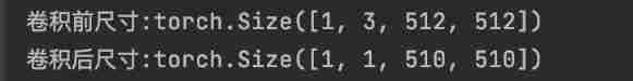

Before convolution , The image size is 512️512, After convolution , The image size is 510️5510. The convolution kernel here is set , Input channel 3, Number of convolution kernels 1, Convolution kernel size 3, nothing padding, Step length is 1, According to the formula above , Output size : （512-3）/1 + 1 = 510

Reference article ：
https://my.oschina.net/u/876354/blog/3064227