[literature translation - Part] revealing the structure of clinical EEG signals by self supervised learning (SSL and RP principles / data / preprocessing)

《Uncovering the structure of clinical EEG signals with
self-supervised learning》 Original address

Intercept the first and second parts （ For RP Method ） Translation

Abstract

The goal is ： Supervised learning paradigms are usually limited by the amount of tag data available . This phenomenon is especially problematic in clinical data , Like electroencephalogram （EEG）, stay EEG in , Tagging can be costly in terms of expertise and human processing time . therefore , Designed to learn EEG The deep learning architecture of data produces a relatively shallow model , At best, its performance is similar to that of traditional feature-based methods . However , in the majority of cases , A large amount of unlabeled data is available . By extracting information from these unlabeled data , Although access to tags is limited , But it is possible to achieve competitive performance through deep neural networks .

Method ： We studied self supervised learning （SSL）, This is a promising technique for discovering structures in unlabeled data , For learning EEG Signal representation . say concretely , We explored two tasks based on temporal context prediction , And the comparative prediction code of two clinical related problems ： be based on EEG Sleep staging and pathological examination . We conducted experiments on two large public data sets with thousands of records , And compared with the methods of pure supervision and manual design .

The main result ： be based on SSL The linear classifier trained by learning features is always better than the pure supervised deep neural network in the state of low labeled data , While achieving competitive performance when all tags are available . Besides , Learning through each method The embedded (embeddings) It reveals physiological and clinical phenomena （ Such as age effect ） Relevant clear underlying structures .

significance ： We demonstrate the benefits of self supervised learning on EEG data . Our results show that ,SSL It may pave the way for the wider use of deep learning models in EEG data .

key word ： Self supervised learning 、 Representational learning 、 machine learning 、 Electroencephalogram 、 Sleep staging 、 Pathological examination 、 Clinical neuroscience

1 Introduce

Electroencephalogram （EEG） And other biological signal modes have been applied in many clinical fields , for example , Study sleep patterns and their disturbances [1], Monitoring seizures [2] And brain - Machine interface [3]. In the last few years , The availability and portability of these devices have increased significantly , It has effectively realized the democratization of use , And unleashed the potential to have a positive impact on people's lives [4,5]. for example , Family sleep staging and apnea testing 、 Pathological EEG detection 、 Applications such as mental load monitoring can now be fully realized .

In all these cases , The monitoring model will produce more and more data to be interpreted . therefore , Need to be able to categorize 、 Test and finally “ understand ” Prediction model of physiological data . Traditionally , This type of modeling relies primarily on a supervisory approach , In the supervision method , A large number of annotated sample datasets are required to train models with high performance .

However , Accurate labeling of physiological data can be expensive 、 Time consuming or impossible . for example , Note sleep recording requires trained technicians to visually view hours of data , And mark them one by one 30 Second window [6]. Clinical records , Such as the record used to diagnose epilepsy or brain injury , Must be reviewed by a neurologist , They may not always be available . More broadly , The noise in the data and the complexity of the brain processes of interest make interpretation and annotation EEG The signal becomes difficult , This leads to a high degree of variability between raters , That's tag noise [7,8]. Besides , In some cases , It may be a challenge to accurately understand the participants' thoughts or behaviors in cognitive neuroscience experiments , This makes it difficult to obtain accurate labels . for example , In imaginary tasks , The subject may not have followed the instructions , Or the research process may be difficult to objectively quantify （ For example, meditation 、 mood ）. therefore , A new paradigm that does not rely primarily on supervised learning is useful for exploiting large unlabeled recordsets （ Such as the recordset generated in the above scenario ） be necessary . However , Traditional unsupervised learning methods （ Such as clustering and potential factor models ） Does not provide a completely satisfactory answer , Because their performance is not as easy to quantify and interpret as a supervised method .

“ Self supervised learning ”（SSL） It's an unsupervised learning method , It learns to represent from unmarked data , Use the structure of the data to provide oversight [9]. By redefining unsupervised learning problem as supervised learning problem ,SSL Allow the use of standard 、 Better understand the optimization process .SSL Include “ auxiliary ” and “ The downstream ” Mission . Downstream tasks are tasks that users are actually interested in , However, the marking is limited or not marked . On the other hand , Auxiliary tasks must be fully relevant to downstream tasks , So that similar representations can be used to perform ; It is important to , You must be able to generate annotations for this auxiliary task using unlabeled data alone .

for example , In computer vision scene , You can use jigsaw puzzles , Extract patches from images , Random scrambling , Then input the neural network , The neural network is trained to restore the original spatial order of the patch [10]. If the network can accomplish this task well , So imagine , It has learned some structures of natural images , And the trained network can solve supervised learning problems on a small scale （ Such as target recognition ） Re used as feature extraction or weight initialization .

In addition to promoting downstream tasks and / Or reduce the number of necessary annotation examples , Self monitoring can also be found to be more common than what is learned in specialized monitoring tasks 、 More robust features [11]. therefore , in consideration of SSL The potential benefits of , It can be used to enhance EEG Your analysis ？

up to now ,SSL Most of its applications are concentrated in the field where there are a lot of annotation data , Like computer vision [9] And natural language processing [12,13]. Especially in computer vision , Deep networks are usually through fully supervised tasks （ for example ,ImageNet Preliminary training ） To train . under these circumstances , There is enough tag data available , In this way, the direct supervised learning of downstream tasks is already competitive [14].SSL In the field where low labeled data patterns are common and the effectiveness of supervised learning is limited , For example, biological signals and EEG Handle , With greater potential . For all that , There is little about SSL And biological signals . These studies either focus on limited downstream tasks and data sets [15], Either in EEG Test their methods on signals other than [16]

therefore , Whether self-monitoring can really improve EEG The standard method of monitoring has yet to be proved , If so , What is the best way to apply it . say concretely , Can we learn through self-monitoring EEG General representation of , And in doing so, reduce the cost of EEG Annotated requirements ？ In view of the deep learning as EEG The growing popularity of processing tools [17], The answer may be right EEG Current practices in the field of processing have had a significant impact . in fact , Although deep learning is known for its data hunger , But the vast majority of all neuroscience research occurs in the field of low labeled data , Including EEG studies ： Clinical studies with hundreds of subjects are often considered big data , Large scale studies are even rarer , It usually comes from the research alliance [18,19,20,21]. therefore , It can be expected that , Most deep learning EEG studies （ Usually in the low tag data state ） The reported performance is still limited so far , And it is not obviously superior to the traditional method [17]. By using unlabeled data ,SSL You can effectively create more examples , So that deep learning can be more successfully applied to EEG.

In this paper , We studied the use of self-monitoring as a general method of learning representations from EEG data . As far as we know , For the first time, we analyzed in detail various types of EEG records SSL Mission . Our goal is to answer the following questions ：

• Good for capturing relevant structures in EEG data SSL What is the task ？
• stay Downstream classification performance aspect ,SSL How does the feature compare to other unsupervised and supervised methods ？
• SSL What are the characteristics of the learned features ？ say concretely ,SSL Whether physiological and clinically relevant structures can be captured from unmarked EEG ？

The rest of the paper is structured as follows . The first 2 Section provides an overview SSL The literature , Then it describes the differences considered in our study SSL Tasks and learning problems . We also introduced the neural structures used in our experiments 、 Baseline methodology and data . Next , The first 3 This section will report the results of our EEG experiments . Last , We will be in the 4 The results are discussed in section .

2 Method

2.1 The most advanced self supervised learning method

Although people don't always think so , but SSL It has been applied in many other fields . In computer vision , Many methods have been proposed , They depend on the spatial structure of the image and the temporal structure of the video . for example , stay [22] in , The context prediction task is used to predict randomly sampled images patch Relative to the second patch The location of , Train the feature extractor on the unlabeled image . This method is used to pre train the neural network , The author reports on Pascal VOC Target detection challenge , Compared with the pure supervision model , Improved performance . These results show for the first time , When limited dimension data is available , Self supervised pre training helps improve performance . Similarly , The puzzle task mentioned above [10] Improve the downstream performance of the same data set . In the field of video processing , The method based on time structure is also proposed ： for example , stay [23] in , Predicting whether the video frame sequence is ordered or unordered is used as an auxiliary task , And test it in the downstream task of human activity identification . Interested readers can visit [9] Find SSL Other applications for images .

Similarly , Modern naturallanguageprocessing （NLP） Tasks usually rely on self-monitoring to learn word embedding , This is at the heart of many applications [24]. for example , The original word2vec The model has been trained , You can predict the words around the headword or predict the headword based on the words around it [12], Then it is reused in various downstream tasks [25]. lately , A kind of Dual task self-monitoring method BERT stay 11 term NLP Mission （ Such as Q & A and named entity recognition ） The state-of-the-art performance [13]. The high performance achieved by this approach demonstrates SSL Potential in learning common representations .

lately , More general ancillary tasks and improved methods have produced powerful results , These results have begun to compete with purely supervisory methods . for example , Compare predictive coding （CPC） It is an autoregressive prediction task in potential space , Successfully used for image 、 Text and voice [11]. Given an encoder and an autoregressive model , Tasks include predicting future windows in the context of a given number of windows （ Or image patches or words ） Encoder output . The author gives some improved results on various downstream tasks ; Follow up studies have further shown that , Higher capacity networks can further improve downstream performance , Especially in low labeled data areas [26]. Momentum contrast （MoCo） Not to propose a new auxiliary task , It's an improvement on the comparison task , That is, the classifier must predict which of two or more inputs is the real sample [27,28]. By improving the sampling of negative samples in the comparison task ,MoCo Helped improve SSL The efficiency of the training and the quality of the representations learned . Similarly , stay [29] Found in , Use the correct data to enhance the transformation （ for example , Random cropping and color distortion on images ） And increasing batch size can significantly improve downstream performance .

after SSL The characteristics of training can be obviously extended to downstream tasks , Therefore, it is necessary to study their statistical structure carefully .Hyvärinen wait forsomeone [30,31] Recently from Nonlinear independent component analysis The point of view formalizes a universal 、 A theoretically sound method . In this broad framework , Use reversible neural networks to embed observations x, And with the auxiliary variable u（ for example , Time index 、segment Index or data history ） Contrast . The discriminator predicts by learning x Is its corresponding auxiliary variable u pairing , Or with disturbance （ Random ） Variable u pairing , Come on x Classify . When the data shows some structure （ for example , Autocorrelation 、 Nonstationarity 、 Non Gaussian ） when , The embeddeds trained in the comparison task will perform recognizable nonlinearity ICA[31]. Most previously introduced SSL Tasks can be viewed through this framework . In view of the wide application of linear independent component analysis as a preprocessing and feature extraction tool in the field of EEG [32,33,34,35], The expansion of the nonlinear field is a natural progress , It may help to improve traditional processing pipeline.

It is worth noting that , Few studies will SSL Applied to biological signals , Although it is possible to exploit large amounts of unlabeled data . stay [15] in , suffer word2vec Inspired the development of a program called wave2vec Model of , Used for processing EEG And ECG （ECG） The time series . By getting from EEG The time-frequency representation of signals and the serial prediction of demographic information are used to learn the characteristics of adjacent windows . However , This method only works on a single EEG The data set has been tested , No benchmarking with fully supervised deep learning methods or expert feature classification .SSL It is also applied to ECG, As a method of learning the characteristics of downstream emotion recognition task ： stay [16] in , A transformation recognition auxiliary task is used , The model must predict which transformations are applied to the original signal . Although these results show the potential of self-regulated learning of biological signals , But it needs to be directed at EEG Of SSL Conduct a broader analysis , Pave the way for practical application .

2.2 Self supervised learning assistant task of EEG

In this section , We will introduce the three used in this article SSL Auxiliary task . The visual explanation of the task is shown in the figure 1 Shown .

2.2.1 Relative positioning (Relative Positioning)

In order to get from multivariable time series $S$ Generate labeled samples in , We suggest For the time window $（x_t,x_{t^{{}^{\prime }}}）$ sampling , Each of these windows $x_t$,$x_{t^{{}^{\prime }}}$ With $R^{C\times T}$ Express ,$T$ Is the duration of each window , The index $t$ Represents the window with $S$ Start time sample . The first window $x_t$ go by the name of “ Anchor window (anchor window)”. Our assumption is , An appropriate representation of the data should evolve slowly over time （ Similar to slow feature analysis （SFA）[36,37] The driving assumptions behind ）, This indicates that the time window should have the same label when closed in time .

for example , In the sleep phase , It usually lasts 1 To 40 minute [38]; therefore , Nearby windows may come from the same sleep stage , The distant window may come from different sleep stages .

Given ${\tau }_{pos}$∈ $N$、 it Control the duration of the positive context , as well as ${\tau }_{neg}$∈ $N$, Corresponds to the negative context around each window , We sample n A marker pair ：


Intuitively speaking , Is all the time index pairs $（t,t^{{}^{\prime }}）$ Set , The size can be from $M$ The size in the time series of is $T$ Window structure of , Given by ${\tau }_{pos}$ and ${\tau }_{neg}$ The duration constraint imposed by a particular choice of . here $y_i\in Y$ Specified by a positive or negative context parameter ：


chart 1 | The three used in this study SSL Visual interpretation of auxiliary tasks . The first column describes the sampling process for obtaining samples in each auxiliary task . The second column describes the training process , Where sample pairs are used Feature extractor $h_{\Theta }$ Do end-to-end training .

We ignore $x_{t^{{}^{\prime }}}$ Not in the anchor window $x_t$ Window pairs in the positive and negative context of . let me put it another way , The label indicates that the two time windows are comparable in time ${\tau }_{pos}$ Closer or better than ${\tau }_{neg}$ further . Notice and [22] The connection of tasks in , We call this auxiliary task “ Relative positioning ”（RP）.

In order to learn how to distinguish time window pairs from each other end to end according to their relative positions , We introduced two functions $h_{\Theta }$ and gRP.$h\Theta ：R^{C\times T}\to R^D$ It's a With parameters Θ Feature extractor , It will window $x$ Map to its representation in feature space . Final , We expect $h_{\Theta }$ Learn the information representation of the original EEG input , This information can be reused in different downstream tasks . And then use Comparison module $g_{RP}$ To aggregate the feature representation of each window . about RP Mission ,$g_{RP}：R^D\times R^D\to R^D$ Combine representations from paired windows by calculating the absolute difference at the element level , from |·| The operator represents ：

$g_{RP}(h_{\Theta }(x),h_{\Theta }(x^{{}^{\prime }}))=|h\Theta (x)-h\Theta (x^{{}^{\prime }})|\in R^D$.

$g_{RP}$ Its function is polymerization $h_{\Theta }$ Feature vectors extracted on two input windows , And highlight their differences , To simplify the comparison task . Last , A coefficient of $w$ Linear context discrimination model $w$∈ $R_D$ And the deviation term $w_0\in R$ Be responsible for forecasting relevant objectives $y$. utilize $g_{RP}$ Predicted binary logic loss , We can take the joint loss function $L（\Theta ,w,w_0）$ It's written in

Let's assume it's for the parameter $（\Theta ,w,w_0）$ It 's completely differentiable . according to $y$ The agreement of , The forecast target is $w^{T}g(h_{\Theta }(x_t),h_{\Theta }(x_t^{{}^{\prime }}))+w_0$ The symbol of .

2.3 Downstream tasks

We discuss two clinical issues that represent current challenges in machine learning based EEG analysis ： Sleep monitoring and pathological screening , An empirical benchmark based on EEG was conducted . These two clinical problems usually lead to classification tasks , Although the number of categories varies , The data generation mechanism is also different ： Sleep monitoring and biological events （ Event level ） of , And pathological screening and population （ Subject level ） Compared with a single patient . These two clinical problems have attracted considerable attention in the research community , This leads to the management of large public databases . In order to make a fair comparison with the supervised method , We are right. 2018 Physiological network challenge in [1,39] and TUH Abnormal EEG [40] Data sets SSL Benchmarking .

First , We have considered Sleep staging , It is a key component of a typical sleep monitoring assessment , Is to diagnose and study sleep disorders （ Such as apnea and narcolepsy ） The key to [41]. machine （ And depth ） Learning literature [42,43,17] Sleep staging has been extensively studied （ About occupy [17] Summary paper 10%）, Although not from SSL From the perspective of . Achieving fully automated sleep staging may have a significant impact on clinical practice , because

1. Consistency among human raters is often limited [7],
2. The annotation process is time-consuming and still largely manual [6].

Sleep staging usually leads to 5 Level classification problem , One of the possible predictions is W（ Wake up the ）、N1、N2、N3（ Different sleep levels ） and R（ Rapid eye movement cycle ）. ad locum , This task includes forecasting the corresponding 30 second EEG The sleep phase of the window .

secondly , We will SSL Applied to pathological examination ：EEG It is routinely used in clinical settings to screen individuals with neurological diseases such as epilepsy and dementia [44,45]. However , Successful pathological examination requires highly specialized medical expertise , Its quality depends on the training and experience of experts . therefore , Automated pathological testing can have a significant impact on clinical practice by promoting neurological screening . This leads to the classification task at the disciplinary level , The challenge is to infer the patient's diagnosis or health status from EEG records . stay TUH Data set , Medical experts mark the records as pathological or non pathological , This leads to the problem of binary classification . It is important to , These two labels reflect a highly heterogeneous situation ： Pathological records may reflect abnormalities caused by various medical conditions , This indicates a fairly complex data generation mechanism . Again , Various supervised methods , Some of them take advantage of deep architecture , In the literature [46,47,48] This task is solved in , Although no method relies on self-monitoring .

When discussing the data used in our experiment , The first 2.6 These two tasks are further described in section .

2.4 Deep learning architecture

In our experiment , We used two different deep learning architectures as embedders $h_{\Theta }$（ See figure for detailed description 2）. Both structures are convolution neural networks composed of spatial and temporal convolution layers , Learn and execute separately EEG Handle typical spatial and temporal filtering operations for pipelines .

first , We call it StagerNet, It is adapted from the previous work on sleep staging , In the window classification of sleep staging , It did well [42].StagerNet It is a three-layer convolutional neural network , Optimization is used to handle 30 Second multichannel EEG window . Contrary to the original architecture ,

1. We use twice as many convolution channels （16 instead of 8）
2. We added batch normalization after two time convolution layers
3. We didn't fill the time convolution
4. We change the dimension of the output layer to D=100, Not the number of classes （ See the picture 2-1）.

This produced a total of 62307 Three trainable parameters .

The second kind , Embedded Architecture ShallowNet Directly from the previous about TUH Literature on outlier data sets [47,48].ShallowNet Originally designed for the brain - Common space mode of filter bank in computer interface （FBCSP） Handle parameterized versions of pipes , It has a single （ Division ） Convolution layer , Then the square nonlinearity 、 Average pool 、 Logarithmic nonlinear and linear output layer . Use batch standardization after time convolution . Simple as it is , But in [48] It shows that , The architecture is in TUH Abnormal data sets perform almost as well as the best model in pathological detection tasks . therefore , We use it as is , In addition to the dimensions of the output layer , We also changed it to D=100（ See the picture 2-2）. This produced a total of 170860 Three trainable parameters .

chart 2 | Neural network structure is used as （1） Sleep EEG and （2） The inserter of pathological examination experiment $h_{\Theta }$.

about CPC Mission $g_{AR}$, We used a hidden layer with a size of $D_{AR}=100$ Of GRU, For experiments on two datasets .

Adam Optimizer [50],${\beta }_1=0.9,{\beta }_2=0.999$, The learning rate is $5\times 10^{-4}$. except CPC Set to 32 Outside , Of all depth models batch The size is set to 256. Training lasts up to 150 Period , Or until the verification loss stops decreasing at least 10 individual epoch（ or CPC Of 6 individual epoch）. With 50% For full connection layer applications dropout, Apply... To trainable parameters of all layers 0.001 Weight decay of . Last , All the parameters of the neural network use uniform He Initialize randomly initialized [51].

2.5 The baseline (Baseline)

SSL The four baseline methods of task and downstream task are compared ：（1） Random weights ,（2） Convolution auto encoder ,（3） Pure supervised learning and （4） Handmade features .

The random weight baseline uses an embedder (embedder), Its weight is frozen after random initialization . Self encoder （AE） It is a more basic representation learning method , The neural network composed of encoder and decoder learns the identity mapping between input and output , for example , Loss of mean square error [52]. ad locum , We use $h_{\Theta }$ As an encoder , A convolutional decoder is designed to invert $h_{\Theta }$ The operation of . The pure supervised model directly trains the downstream classification problem , That is, it can access the marked data . So , We added an additional linear classification layer to the embedder , Then the whole model is trained by using multi class cross entropy loss .

Last , We also include traditional machine learning baselines based on manual features .

For sleep staging , We extracted the following features [42]： mean value 、 variance 、 skewness 、 kurtosis 、 standard deviation 、 Frequency logarithmic power band （0.5、4.5、8.5、11.5、15.5、30）Hz Between , And all possible ratio 、 Peak to peak 、 Hurst index 、 Approximate entropy and Hjorth Complexity . This leads to every EEG Channels have 37 Features , These features are connected into a vector . If the artifact causes the missing value in the window eigenvector , We use the Characteristic average Estimate missing values in a characteristic way .

For pathological examination , Such as [48] Described in , Riemannian geometric features are used , As report goes , The nonlinear classifier based on tangent space feature training is applied in TUH High accuracy is achieved on the evaluation set of abnormal data set . We do not average the covariance matrix for each record , So as to make a fair comparison with the methods of other windows . therefore , For EEG C passageway , The input of the classifier has dimension $C（C+1）/2$.

For downstream tasks , adopt RP、TS、CPC and AE The characteristics of learning use L2 Regularization parameters C=1 Linear logistic regression To classify , and Handmade features Then use Random forest classifier To classify , The classifier contains 300 tree , Maximum depth is 15 Tree , The maximum number of features of each tree is $\sqrt{F}$（ among F Number of features is ）. Balance accuracy （bal acc） Defined as the average of each class recall, Model performance for evaluating downstream tasks . Besides , During training , Losses are weighted to account for class imbalances . Use braindecode[53]、MNE Python[54]、Pytork[55]、pyRiemann[56] and scikit learn[57] The software package trains the model . Last , Deep learning model in 1 or 2 individual Nvidia Tesla V100 GPU Training on , Time ranges from a few minutes to 7 Hours don't wait , It depends on the amount of data 、 Early stop and GPU To configure .

2.6 data

The experiment was conducted in two public EEG On the dataset , As shown in the table 1 And table 2 Shown .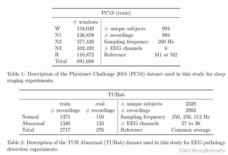

2.6.1 Physionet Challenge 2018 dataset

First , We are Physionet Challenge 2018（PC18） Data sets [1,39] The sleep staging experiment was carried out on . This data set was originally released in the context of an open source competition , The competition aims to detect arousal in sleep records , A brief waking moment at night . Yes 1983 name （ Suspected ） Nighttime monitoring for patients with sleep apnea , And measure their EEG、EOG、 chin EMG、 Respiratory airflow and oxygen saturation . To be specific , The international 10/20 Systematic 6 individual EEG Channel in 200 Hz Make a note of ：F3-M2、F4-M1、C3-M2、C4-M1、O1-M2 and O2-M1. then ,7 Trained scorers according to AASM manual [58] Annotate the recorded data to sleep stage （W、N1、N2、N3 and R）. Besides , The record also found 9 There are different types of awakening and 4 There are three types of sleep apnea events . Since the sleep phase is marked only in about half of the records （ Used as a training set during the competition ） Go public , We will focus our analysis on this 994 On a record . In this part of the data , The average age is 55 year （ The minimum 18 year , The highest 93 year ）,33% Of the participants were women .

2.6.2 TUH Abnormal EEG dataset

We used TUH Abnormal EEG data set V2.0.0（TUHab） Conduct Pathological EEG detection experiment [40]. The dataset is [19] A subset of , contain 2329 Of different patients who underwent clinical EEG examination in hospital 2993 Time 15 Minutes or more . According to the detailed doctor's report , Each record is marked as “ normal ”（1385 Time record ） or “ abnormal ”（998 Time record ）. The sampling frequency for most records is 250 Hz（ Although some records are sampled at 256 or 512 Hz）, contain 27 To 36 An electrode . Besides , The corpus is divided into a training set and an evaluation set , Each training set and evaluation set has 2130 Secondary sum 253 Time record . The average age of all records is 49.3 year （ Minimum 1 year , Maximum 96 year ）,53.5% Of the patients were female patients .

2.6.3 Data splitting and sampling

We will PC18 and TUHab The available records are divided into training 、 Verification and test sets , So that the samples in each record are in only one set （ See table 3）.

about PC18, We used 60-20-20% Random segmentation of , It means training 、 The verification and test sets have 595、199 and 199 Time record . about RP and TS, Extract from each record 2000 Or three pairs of windows . about CPC, Extracted from each record batch The number is calculated as the number of windows in the record 0.05 times ; Besides , We will batch The size is set to 32.

about TUHab, We use the evaluation set provided as the test set . Development set records are divided into 80-20% Training set and verification set . therefore , We are training 、 Verification and testing are concentrated on 2171、543 and 276 Time record . because TUHab The record of is short , We randomly selected 400 individual RP Yes or TS triplets , Not in every record 2000 individual . We used and PC18 same CPC Sampling parameters .

2.6.4 Data preprocessing

Of these two data sets EEG Record preprocessing is different .

stay PC18 On , First use the with Hamming window 30 Hz FIR low pass filter Original EEG Filtering , With a higher frequency of rejecting sleep staging as unimportant [42,59]. And then EEG passageway Down sampling to 100Hz, To reduce the dimension of input data . For the same reason , We will focus our analysis on the channel F3-M2 and F4-M1 On . Last , The extraction size is 30 second （3000 x 2） Non overlapping windows of .

stay TUHab On , Used with [48] Similar procedures described in . The first minute of each recording tailoring , To delete noisy data at the beginning of recording . Longer files are also cropped , In this way, each recording can be used at most 20 minute . then , All recordings have been selected 21 Channels （Fp1、Fp2、F7、F8、F3、Fz、F4、A1、T3、C3、Cz、C4、T4、A2、T5、P3、Pz、P4、T6、O1 and O2）. take EEG passageway Down sampling to 100 Hz, and stay ±800µV There's a cut , To reduce the impact of large false deviations in the original data . Extract non overlapping 6-s window , The magnitude is 600×21 The window of .

Last , The amplitude between peaks in the two data sets is less than 1µV Windows of are rejected . The rest of the windows proceed by channel Standardization , The mean and unit standard deviation are zero .

3 Code

I can't get out ！！！！ Routine address

#  Use SSL-Relative Positioning Yes EEG Signal sleep staging 
# Written By FelicityXu
# 20220226
import os

import numpy as np
import torch
from braindecode import EEGClassifier
from braindecode.datasets import SleepPhysionet, BaseConcatDataset
from braindecode.models import SleepStagerChambon2018
from braindecode.preprocessing import Preprocessor, scale, preprocess, create_windows_from_events
from braindecode.samplers import RelativePositioningSampler
from braindecode.util import set_random_seeds
from sklearn.linear_model import LogisticRegression
from sklearn.metrics import balanced_accuracy_score, confusion_matrix, classification_report
from sklearn.model_selection import train_test_split
from sklearn.pipeline import make_pipeline
from sklearn.preprocessing import scale as standard_scale, StandardScaler
from skorch.callbacks import Checkpoint, EarlyStopping, EpochScoring
from skorch.helper import predefined_split
from torch import nn
#
# import sys
#
# sys.setrecursionlimit(1000000)
from torch.utils.data import DataLoader

random_state = 87
n_jobs = 1

'''  load SleepPhysionet Data sets  '''
# crop_wake_mins：Number of minutes of wake time to keep before
# the first sleep event and after the last sleep event.
# Used to reduce the imbalance in this dataset. Default of 30 mins.
dataset = SleepPhysionet(
    subject_ids=[0, 1, 2], recording_ids=[1], crop_wake_mins=30)

'''  Data preprocessing  '''
#  Next , We preprocess the raw data .
#  We convert the data to microvolts and apply a low-pass filter . because Sleep Physionet The data has been in the form of  100 Hz  sampling , We do not need to apply resampling .
high_cut_hz = 30

preprocessors = [
    Preprocessor(scale, factor=1e6, apply_on_array=True),
    Preprocessor('filter', l_freq=None, h_freq=high_cut_hz, n_jobs=n_jobs)

]

#  Data preprocessing 
preprocess(dataset, preprocessors)

'''  Extract window   We extract  30  Second window for auxiliary and downstream tasks .  because RP（ And general  SSL） No need to tag data , So you can use braindecode.datautil.windower.create_fixed_length_window().  However , ad locum , Purely for convenience , We directly extract the marked window , So that we can reuse them later in the sleep phasing downstream tasks . '''


window_size_s = 30
sfreq = 100
window_size_samples = window_size_s * sfreq  #  How many sample points are there in the window 

mapping = {
      # We merge stages 3 and 4 following AASM standards.
    'Sleep stage W': 0,
    'Sleep stage 1': 1,
    'Sleep stage 2': 2,
    'Sleep stage 3': 3,
    'Sleep stage 4': 3,
    'Sleep stage R': 4,
}

windows_dataset = create_windows_from_events(
    dataset, trial_start_offset_samples=0, trial_stop_offset_samples=0,
    window_size_samples=window_size_samples,
    window_stride_samples=window_size_samples, preload=True, mapping=mapping
)

#  Preprocessing window  z-score normalization 
preprocess(windows_dataset, [Preprocessor(standard_scale, channel_wise=True)])

'''  Split the data into training sets 、 Verification set and test set   We will record by subject Randomly divided into training sets 、 Validation set and test set .  We further define a new  Dataset  class , It can receive a pair of indexes and return to the corresponding window .  When training and evaluating auxiliary tasks , This will be necessary . '''

subjects = np.unique(windows_dataset.description['subject'])  #  Remove duplicate numbers from the array , Output after sorting 
subj_train, subj_test = train_test_split(
    subjects, test_size=0.4, random_state=random_state)
subj_valid, subj_test = train_test_split(
    subjects, test_size=0.5, random_state=random_state)


class RelativePositioningDataset(BaseConcatDataset):
    """BaseConcatDataset with __getitem__ that expects 2 indices and a target. """
    def __init__(self, list_of_ds):
        super().__init__(list_of_ds)  #  Associate a parent class with a subclass , Calling the __init__ Method , Let the instance contain all the properties of the parent class 
        self.return_pair = True

    def __getitem__(self, index):
        if self.return_pair:
            ind1, ind2, y = index
            return(super().__getitem__(ind1)[0],
                   super().__getitem__(ind2)[0]), y
        else:
            return super().__getitem__(index)

    @property #  Modification methods , Methods can be accessed like properties 
    def return_pair(self):
        return self.return_pair

    @return_pair.setter # @*.setter  Allow you to use @property Decorated function assignment ：
    def return_pair(self, value):
        self._return_pair = value


split_ids = {
    'train': subj_train, 'valid': subj_valid, 'test': subj_test}
splitted = dict()
for name, values in split_ids.items():  # name:"train" "valid" "test"
    splitted[name] = RelativePositioningDataset(
        [ds for ds in windows_dataset.datasets
         if ds.description['subject'] in values])


'''  Create samplers   Next , We need to create a sampler . These samplers will be used to randomly sample pairs of samples , To train and validate our model through self-monitoring . RP  The sampler has two main superparameters .tau_pos and tau_neg  , respectively,   control “ just ” and “ negative ” The size of the context .  Be less than tau_pos Sample delimited window pairs will be tagged 1, And be surpassed  tau_neg Sample delimited window pairs will be tagged 0.  ad locum , We use and 1 The same value in , namely ` tau_pos`= 1  Minutes and ` tau_neg`= 15  minute .  The sampler also controls the number of logarithms to be sampled （ Use  n_examples Definition ）.  This number can be very large , To help standardize auxiliary task training , For example, each record  2,000  Yes   ad locum , We use less each time  250  Yes, to reduce training time . '''
tau_pos, tau_neg = int(sfreq * 60), int(sfreq * 15 * 60)  #  Size of positive and negative context sampling points 
n_examples_train = 250 * len(splitted['train'].datasets)
n_examples_valid = 250 * len(splitted['valid'].datasets)
n_examples_test = 250 * len(splitted['test'].datasets)

train_sampler = RelativePositioningSampler(
    splitted['train'].get_metadata(), tau_pos=tau_pos, tau_neg=tau_neg,
    n_examples=n_examples_train, same_rec_neg=True, random_state=random_state)
valid_sampler = RelativePositioningSampler(
    splitted['valid'].get_metadata(), tau_pos=tau_pos, tau_neg=tau_neg,
    n_examples=n_examples_valid, same_rec_neg=True,
    random_state=random_state).presample()
test_sampler = RelativePositioningSampler(
    splitted['test'].get_metadata(), tau_pos=tau_pos, tau_neg=tau_neg,
    n_examples=n_examples_test, same_rec_neg=True,
    random_state=random_state).presample()

'''  Create a deep learning model .  Use 4 A modified version of the sleep hierarchy described in —— A four layer convolutional neural network —— As our embedder .  We change the dimension of the last layer to get  100  Dimension embedding , Use  16  A convolution channel instead of  8  individual , And add batch normalization after two time convolution layers .  We use the following definition  # ContrastiveNet Class further wraps the model into a connected architecture . This enables us to train feature extractors end-to-end . '''
# device = 'cuda' if torch.cuda.is_available() else 'cpu'
device = 'cpu'
# if device == 'cuda':
# torch.backends.cudnn.benchmark = True

set_random_seeds(seed=random_state, cuda=device == 'cuda')

# Extract number of channels and time steps from dataset
n_channels, input_size_samples = windows_dataset[0][0].shape
emb_size = 100

#  come from  Chambon  wait forsomeone  2018  Sleep staging architecture .
emb = SleepStagerChambon2018(
    n_channels,
    sfreq,
    n_classes=emb_size,
    n_conv_chs=16,
    input_size_s=input_size_samples / sfreq,
    dropout=0,
    apply_batch_norm=True
)


class ContrastiveNet(nn.Module):
    """Contrastive module with linear layer on top of siamese embedder. Parameters ---------- emb : nn.Module Embedder architecture. emb_size : int Output size of the embedder. dropout : float Dropout rate applied to the linear layer of the contrastive module. """
    def __init__(self, emb, emb_size, dropout=0.5):
        super().__init__()
        self.emb = emb
        self.clf = nn.Sequential(
            nn.Dropout(dropout),
            nn.Linear(emb_size, 1)
        )

    def forward(self, x):
        x1, x2 = x
        z1, z2 = self.emb(x1), self.emb(x2)
        return self.clf(torch.abs(z1 - z2)).flatten()


model = ContrastiveNet(emb, emb_size).to(device)


'''  Training   We can now train our network on ancillary tasks .  We use and 1 A similar super parameter in , But less  epoch  And improve the learning rate , To address the smaller settings of this sample . '''
lr = 5e-3
batch_size = 512
n_epochs = 25
num_workers = 0 if n_jobs <= 1 else n_jobs

cp = Checkpoint(dirname='', f_criterion=None, f_optimizer=None, f_history=None)
early_stopping = EarlyStopping(patience=10)
train_acc = EpochScoring(
    scoring='accuracy', on_train=True, name='train_acc', lower_is_better=False)
valid_acc = EpochScoring(
    scoring='accuracy', on_train=False, name='valid_acc',
    lower_is_better=False)
callbacks = [
    ('cp', cp),
    ('patience', early_stopping),
    ('train_acc', train_acc),
    ('valid_acc', valid_acc)
]

clf = EEGClassifier(
    model,
    criterion=torch.nn.BCEWithLogitsLoss,
    optimizer=torch.optim.Adam,
    max_epochs=n_epochs,
    iterator_train__shuffle=False,
    iterator_train__sampler=train_sampler,
    iterator_valid__sampler=valid_sampler,
    iterator_train__num_workers=num_workers,
    iterator_valid__num_workers=num_workers,
    train_split=predefined_split(splitted['valid']),
    optimizer__lr=lr,
    batch_size=batch_size,
    callbacks=callbacks,
    device=device
)
# Model training for a specified number of epochs. `y` is None as it is already
# supplied in the dataset.
clf.fit(splitted['train'], y=None)
clf.load_params(checkpoint=cp)  # Load the model with the lowest valid_loss

os.remove('./params.pt')  # Delete parameters file

'''  Sleep staging using the representation of learning   We can now use a trained convolutional neural network as a feature extractor .  We use a linear logistic regression classifier to perform sleep stage classification from the learned feature representation . '''
# Extract features with the trained embedder
data = dict()
for name, split in splitted.items():
    split.return_pair = False  # Return single windows
    loader = DataLoader(split, batch_size=batch_size, num_workers=num_workers)
    with torch.no_grad():
        feats = [emb(batch_x.to(device)).cpu().numpy()
                 for batch_x, _, _ in loader]
    data[name] = (np.concatenate(feats), split.get_metadata()['target'].values)

# Initialize the logistic regression model
log_reg = LogisticRegression(
    penalty='l2', C=1.0, class_weight='balanced', solver='lbfgs',
    multi_class='multinomial', random_state=random_state)
clf_pipe = make_pipeline(StandardScaler(), log_reg)

# Fit and score the logistic regression
clf_pipe.fit(*data['train'])
train_y_pred = clf_pipe.predict(data['train'][0])
valid_y_pred = clf_pipe.predict(data['valid'][0])
test_y_pred = clf_pipe.predict(data['test'][0])

train_bal_acc = balanced_accuracy_score(data['train'][1], train_y_pred)
valid_bal_acc = balanced_accuracy_score(data['valid'][1], valid_y_pred)
test_bal_acc = balanced_accuracy_score(data['test'][1], test_y_pred)

print('Sleep staging performance with logistic regression:')
print(f'Train bal acc: {
      train_bal_acc:0.4f}')
print(f'Valid bal acc: {
      valid_bal_acc:0.4f}')
print(f'Test bal acc: {
      test_bal_acc:0.4f}')

print('Results on test set:')
print(confusion_matrix(data['test'][1], test_y_pred))
print(classification_report(data['test'][1], test_y_pred))