当前位置:网站首页>Swing transformer details-1
Swing transformer details-1
2022-07-03 10:00:00 【Star soul is not a dream】
Catalog
1. Patch Partition + Liner Embedding modular
2. Swin Transformer block( A complete W-MSA)
Add ( Look directly if you are familiar with it 3. Patch Merging)
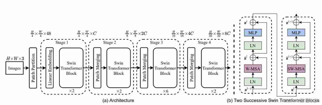
(b) Two consecutive Swin Transformer Blocks( See formula for symbols (3)).W-MSA and SW-MSA There are rules (regular) Window configuration and movement (shifted) Window configuration multi-head self attention modules.
Source code :
 https://github.com/microsoft/Swin-Transformer
1. Patch Partition + Liner Embedding modular
Code :
class PatchEmbed(nn.Module):
    r""" Image to Patch Embedding

    Args:
        img_size (int): Image size.  Default: 224.
        patch_size (int): Patch token size. Default: 4.
        in_chans (int): Number of input image channels. Default: 3.
        embed_dim (int): Number of linear projection output channels. Default: 96.
        norm_layer (nn.Module, optional): Normalization layer. Default: None
    """

    def __init__(self, img_size=224, patch_size=4, in_chans=3, embed_dim=96, norm_layer=None):
        super().__init__()
        img_size = to_2tuple(img_size)
        patch_size = to_2tuple(patch_size)
        patches_resolution = [img_size[0] // patch_size[0], img_size[1] // patch_size[1]]
        self.img_size = img_size
        self.patch_size = patch_size
        self.patches_resolution = patches_resolution
        self.num_patches = patches_resolution[0] * patches_resolution[1]

        self.in_chans = in_chans
        self.embed_dim = embed_dim

        self.proj = nn.Conv2d(in_chans, embed_dim, kernel_size=patch_size, stride=patch_size)
        if norm_layer is not None:
            self.norm = norm_layer(embed_dim)
        else:
            self.norm = None

    def forward(self, x):
        B, C, H, W = x.shape
        # FIXME look at relaxing size constraints
        assert H == self.img_size[0] and W == self.img_size[1], \
            f"Input image size ({H}*{W}) doesn't match model ({self.img_size[0]}*{self.img_size[1]})."
        x = self.proj(x).flatten(2).transpose(1, 2)  # B Ph*Pw C
        if self.norm is not None:
            x = self.norm(x)
        return x

    def flops(self):
        Ho, Wo = self.patches_resolution
        flops = Ho * Wo * self.embed_dim * self.in_chans * (self.patch_size[0] * self.patch_size[1])
        if self.norm is not None:
            flops += Ho * Wo * self.embed_dim
        return flops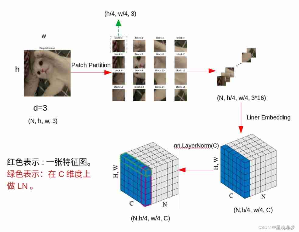

here ,Patch Partition + Liner Embedding Through nn.Conv2d, take kernel_size and stride Set to patch_size( Divide the image into several pieces , Here for 4) size . It's really just a 2d Convolution implementation of the sliding window . then , In order to be in the channel dimension C( In the code is 96) Conduct LayerNorm, the flatten(2).transpose(1,2) # (B h/4 * w/4 C). In the picture above N Batch size B.
Realization :
self.proj = nn.Conv2d(in_chans, embed_dim, kernel_size=patch_size, stride=patch_size) #  Realization 4 Block partition , And will dim  To embed_dim
if norm_layer is not None:
    self.norm = norm_layer(embed_dim)
else:
    self.norm = None


B, C, H, W = x.shape #  Input image Of size
x = self.proj(x).flatten(2).transpose(1, 2)  # B Ph*Pw C  Because it needs to be right C do LN
if self.norm is not None:
    x = self.norm(x)
2. Swin Transformer block( A complete W-MSA)
Don't think about it first cyclic shift.
partition windows
window partition The function is used to divide the tensor into windows according to the specified window size . Change the original tensor from B H W C, Divide into num_windows*B, window_size, window_size, C, among num_windows = H*W / (window_size*window_size), That is, the number of windows .


Code :
def window_partition(x, window_size):
    """
    Args:
        x: (B, H, W, C)
        window_size (int): window size

    Returns:
        windows: (num_windows*B, window_size, window_size, C)
    """
    B, H, W, C = x.shape
    x = x.view(B, H // window_size, window_size, W // window_size, window_size, C)
    windows = x.permute(0, 1, 3, 2, 4, 5).contiguous().view(-1, window_size, window_size, C)
    return windows
x_windows: (nW*B, window_size, window_size, C )
(nW*B, window_size*window_size, C)
 (nW*B, window_size*window_size, C)
W-MSA
# W-MSA/SW-MSA
attn_windows = self.attn(x_windows, mask=self.attn_mask) # nW*B, window_size*window_size, C
there mask Indicates whether it is necessary to calculate self-attention Time mask . The following discussion does not take mask Of MSA.
self.attn = WindowAttention(
            dim,                                      #  Number of input channels
            window_size=to_2tuple(self.window_size),  #  Become two tuples , such as 7 become (7,7)
            num_heads=num_heads,                      #  Number of heads of attention
            qkv_bias=qkv_bias,                        # (bool,  Optional ): If True, add a learnable bias to query, key, value. Default: True
            qk_scale=qk_scale,                        # (float | None,  Optional ): Override default qk scale of head_dim ** -0.5 if set.
            attn_drop=attn_drop,                      # Attention dropout rate. Default: 0.0
            proj_drop=drop)                           # Stochastic depth rate. Default: 0.0
class WindowAttention(nn.Module) in
def forward(self, x, mask=None):
    """
    Args:
        x: input features with shape of (num_windows*B, N, C) (nW*B, window_size*window_size, C)
        mask: (0/-inf) mask with shape of (num_windows, Wh*Ww, Wh*Ww) or None
    """
    B_, N, C = x.shape # (nW*B, window_size*window_size, C)
    qkv = self.qkv(x).reshape(B_, N, 3, self.num_heads, C // self.num_heads).permute(2, 0, 3, 1, 4)
    q, k, v = qkv[0], qkv[1], qkv[2]  # make torchscript happy (cannot use tensor as tuple)

    q = q * self.scale
    attn = (q @ k.transpose(-2, -1))
self.qkv = nn.Linear(dim, dim * 3, bias=qkv_bias) # qkv_bias=True(nW*B, window_size*window_size, C)
(nW*B, window_size*window_size, 3C)
(nW*B, window_size*window_size, 3, num_heads, C // num_heads)
qkv: (3, nW*B, num_heads, window_size*window_size, C // num_heads)
 (nW*B, window_size*window_size, 3C)
 qkv: (3, nW*B, num_heads, window_size*window_size, C // num_heads)
Here stage 1,2,3,4 Of Swin Transformer block Of num_heads Respectively [3, 6, 12, 24]. here C At every Swin Transformer block Will double , and num_heads Also double . so q, k, v Of C // num_heads Is a fixed value . hypothesis Patch Partition + Liner Embedding Module output C by 96, be C // num_heads Fixed for 32.
q,k,v Dimensions (nW*B, num_heads, window_size*window_size, C // num_heads).
Do it in each drawn window self-attention. for example , The window is 7, In total 7*7 = 49 Elements , Each element will do 49 Time self-attention , So the output is (49 ,49) size .
head_dim = dim // num_heads

self.scale = qk_scale or head_dim ** -0.5 # qk_scale = None ,  1/sqrt(d)
q: (nW*B, num_heads, window_size*window_size, C // num_heads) * 1/sqrt(head_dim)
k.transpose(-2, -1): (nW*B, num_heads, C // num_heads,window_size*window_size)
= attn: (nW*B, num_heads, window_size*window_size, window_size*window_size)
 k.transpose(-2, -1): (nW*B, num_heads, C // num_heads,window_size*window_size)
Relative position deviation
Above picture , Red is the relative position deviation . In the paper ,Q,K,V dimension :(window_size*window_size, C // num_heads). and B The dimensions are :(window_size*window_size, window_size*window_size).
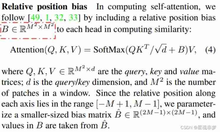
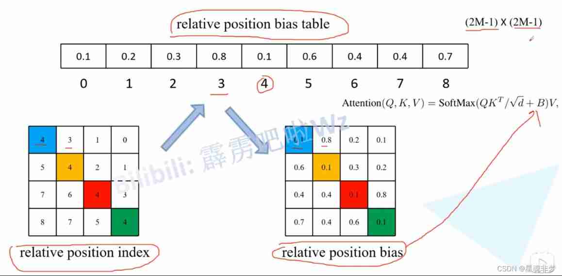
The example here is M = window_size = 2. Relative position deviation B It's through Relative position index check Relative position deviation table ( In the paper  ) Got . The relative position index is based on M Fixed size , The relative position deviation table is obtained by training .
So how to get the relative position index ?
hypothesis M = window_size = 2.

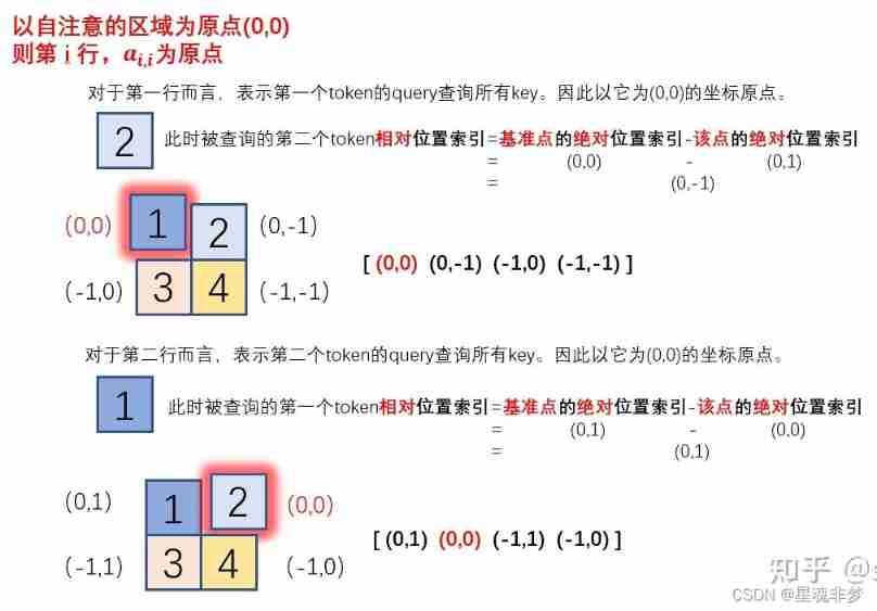
Because ultimately we want to use one-dimensional position coordinates x+y Instead of two-dimensional position coordinates (x,y), for fear of (0,-1) (-1,0) When the two coordinates are converted into one dimension, it is -1, After us Index relative positions Some of it went on linear transformation , Make it possible to pass A one-dimensional The position coordinates of The only mapping To a A two-dimensional The position coordinates of .
Why? Relative position index Yes (2M-1) * (2M-1) States , And why The length of the relative position deviation table is (2M-1) * (2M-1)?
Relative position index The value range of is [-M + 1, M-1], So coordinates ( That's ok , Column ) Values are (2M-1) States . Such as M = 2, Then the coordinates ( That's ok , Column ) The value range is [-1, 1], Yes 3 States , So the total is 9 States .
therefore The length of the relative position deviation table is (2M-1) * (2M-1) .
Realization :
window_size = (2, 2)
# get pair-wise relative position index for each token inside the window
coords_h = torch.arange(window_size[0])
coords_w = torch.arange(window_size[1])
coords = torch.meshgrid([coords_h, coords_w])
# tensor([[0, 0],
# [1, 1]]),
# tensor([[0, 1],
# [0, 1]])
coords = torch.stack(coords) # 2, Wh, Ww
# tensor([[[0, 0],
# [1, 1]],
# [[0, 1],
# [0, 1]]])
coords_flatten = torch.flatten(coords, 1) # 2, Wh*Ww
# tensor([[0, 0, 1, 1],
# [0, 1, 0, 1]])
relative_coords_first = coords_flatten[:, :, None] # 2, wh*ww, 1
# tensor([[[0],
# [0],
# [1],
# [1]],
# [[0],
# [1],
# [0],
# [1]]])
relative_coords_second = coords_flatten[:, None, :] # 2, 1, wh*ww
# tensor([[[0, 0, 1, 1]],
# [[0, 1, 0, 1]]])
relative_coords = relative_coords_first - relative_coords_second # 2, Wh*Ww, Wh*Ww # Broadcast the elements of the former to subtract
# tensor([[[ 0, 0, -1, -1],
# [ 0, 0, -1, -1],
# [ 1, 1, 0, 0],
# [ 1, 1, 0, 0]], # x ( That's ok ) coordinate
# [[ 0, -1, 0, -1],
# [ 1, 0, 1, 0],
# [ 0, -1, 0, -1],
# [ 1, 0, 1, 0]]]) # y( Column ) coordinate
relative_coords = relative_coords.permute(1, 2, 0).contiguous() # Wh*Ww, Wh*Ww, 2 # 2 Express (x, y) coordinate namely ( That's ok , Column )
# tensor([[[ 0, 0], # Each pair is one (x, y) coordinate
# [ 0, -1],
# [-1, 0],
# [-1, -1]],
# [[ 0, 1],
# [ 0, 0],
# [-1, 1],
# [-1, 0]],
# [[ 1, 0],
# [ 1, -1],
# [ 0, 0],
# [ 0, -1]],
# [[ 1, 1],
# [ 1, 0],
# [ 0, 1],
# [ 0, 0]]])
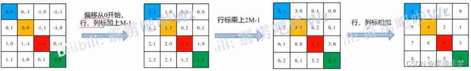
relative_coords[:, :, 0] += window_size[0] - 1 # shift to start from 0 # * (M-1)
# tensor([[[ 1, 0], # all x ( That's ok ) The coordinates are from 0 Start
# [ 1, -1],
# [ 0, 0],
# [ 0, -1]],
# [[ 1, 1],
# [ 1, 0],
# [ 0, 1],
# [ 0, 0]],
# [[ 2, 0],
# [ 2, -1],
# [ 1, 0],
# [ 1, -1]],
# [[ 2, 1],
# [ 2, 0],
# [ 1, 1],
# [ 1, 0]]])
relative_coords[:, :, 1] += window_size[1] - 1 # all y( Column ) The coordinates are from 0 Start # * (M-1)
# tensor([[[1, 1],
# [1, 0],
# [0, 1],
# [0, 0]],
# [[1, 2],
# [1, 1],
# [0, 2],
# [0, 1]],
# [[2, 1],
# [2, 0],
# [1, 1],
# [1, 0]],
# [[2, 2],
# [2, 1],
# [1, 2],
# [1, 1]]])
relative_coords[:, :, 0] *= 2 * window_size[1] - 1 # x ( That's ok ) coordinate * (2M -1) # Wh*Ww, Wh*Ww, 2
# tensor([[[3, 1],
# [3, 0],
# [0, 1],
# [0, 0]],
# [[3, 2],
# [3, 1],
# [0, 2],
# [0, 1]],
# [[6, 1],
# [6, 0],
# [3, 1],
# [3, 0]],
# [[6, 2],
# [6, 1],
# [3, 2],
# [3, 1]]])
relative_position_index = relative_coords.sum(-1) # Wh*Ww, Wh*Ww
# tensor([[4, 3, 1, 0], # (x, y) coordinate -> Sum becomes 1-d
# [5, 4, 2, 1],
# [7, 6, 4, 3],
# [8, 7, 5, 4]])
# self.register_buffer("relative_position_index", relative_position_index) # Register as a variable that does not participate in online learning relative_position_index = relative_position_index.view(-1)
# tensor([4, 3, 1, 0, 5, 4, 2, 1, 7, 6, 4, 3, 8, 7, 5, 4])
num_heads = 1
relative_position_bias_table = torch.zeros((2 * window_size[0] - 1) * (2 * window_size[1] - 1), num_heads) # 2*Wh-1 * 2*Ww-1, nH
trunc_normal_(relative_position_bias_table, std=.02) # truncation Normal distribution relative_position_bias_table Parameters for training nn.Parameter
# tensor([[ 0.0121],
# [-0.0030],
# [ 0.0043],
# [ 0.0263],
# [ 0.0264],
# [ 0.0187],
# [ 0.0364],
# [ 0.0182],
# [-0.0170]])
relative_position_value = relative_position_bias_table[relative_position_index] # Wh*Ww * Wh*Ww, nH Look up the table
relative_position_bias = relative_position_value.view(window_size[0] * window_size[1], window_size[0] * window_size[1], -1) # Wh*Ww,Wh*Ww,nH
relative_position_bias = relative_position_bias.permute(2, 0, 1).contiguous() # nH, Wh*Ww, Wh*Ww
relative_position_bias = relative_position_bias.unsqueeze(0) # 1, nH, Wh*Ww, Wh*Wwattn = attn + relative_position_bias # Yes relative_position_bias Broadcast to add element by element # (nW*B, num_heads, window_size*window_size, window_size*window_size)
# Don't think about it first mask
self.attn_drop = nn.Dropout(attn_drop) #attn_drop: Dropout ratio of attention weight. Default: 0.0
attn = self.softmax(attn)
attn = self.attn_drop(attn)
x = (attn @ v).transpose(1, 2).reshape(B_, N, C)
x = self.proj(x) # nn.Linear(dim, dim)
x = self.proj_drop(x) # nn.Dropout(proj_drop) Default: 0.0
attn: (nW*B, num_heads, window_size*window_size, window_size*window_size)
(nW*B, window_size*window_size, num_heads, C // num_heads)
(nW*B, window_size*window_size, C)
attn_windows: (nW*B, window_size*window_size, C)
 (nW*B, window_size*window_size, num_heads, C // num_heads)
  (nW*B, window_size*window_size, C)
  attn_windows: (nW*B, window_size*window_size, C)
merge windows
# merge windows
attn_windows = attn_windows.view(-1, self.window_size, self.window_size, C)
shifted_x = window_reverse(attn_windows, self.window_size, H, W)  # B H' W' C   The first one here Transformer:H=W=56
attn_windows: (nW*B, window_size*window_size, C)
(nW*B, window_size, window_size, C)
(B, H, W, C)
 (nW*B, window_size, window_size, C)
  (B, H, W, C)
def window_reverse(windows, window_size, H, W):
    """
    Args:
        windows: (num_windows*B, window_size, window_size, C) # num_windows*B = H*W / (window_size*window_size) *B
        window_size (int): Window size
        H (int): Height of image  # 224/4 = 56/[1,2,2^2, 2^3]
        W (int): Width of image

    Returns:
        x: (B, H, W, C)
    """
    B = int(windows.shape[0] / (H * W / window_size / window_size)) #  Batch size
    x = windows.view(B, H // window_size, W // window_size, window_size, window_size, -1) # (B, H // window_size, W // window_size, window_size, window_size, C)
    x = x.permute(0, 1, 3, 2, 4, 5).contiguous().view(B, H, W, -1) # (B, H, W, C)
    return x
Don't think about it first reverse cyclic shift, See below .
(B, H, W, C)
# FFN
x = shortcut + self.drop_path(x) # (B, H*W, C)
x = x + self.drop_path(self.mlp(self.norm2(x)))
MLP
mlp_ratio=4.
act_layer=nn.GELU
mlp_hidden_dim = int(dim * mlp_ratio)
self.mlp = Mlp(in_features=dim, hidden_features=mlp_hidden_dim, act_layer=act_layer, drop=drop)
class Mlp(nn.Module):
def __init__(self, in_features, hidden_features=None, out_features=None, act_layer=nn.GELU, drop=0.):
super().__init__()
out_features = out_features or in_features
hidden_features = hidden_features or in_features
self.fc1 = nn.Linear(in_features, hidden_features)
self.act = act_layer()
self.fc2 = nn.Linear(hidden_features, out_features)
self.drop = nn.Dropout(drop)
def forward(self, x):
x = self.fc1(x)
x = self.act(x)
x = self.drop(x)
x = self.fc2(x)
x = self.drop(x)
return xAdd ( Look directly if you are familiar with it 3. Patch Merging)
among ,shortcut:(B, H*W, C). There is one self.drop_path(x) operation .
self.drop_path = DropPath(drop_path) if drop_path > 0. else nn.Identity()torch.nn.identity() Methods, _sigmoidAndReLU The blog of -CSDN Blog _torch.nn.identity()
nn.Identity() : For occupancy , Do nothing .
DropPath:DropPath - Bashu scholar - Blog Garden
Realization :
def drop_path(x, drop_prob: float = 0., training: bool = False, scale_by_keep: bool = True):
    """Drop paths (Stochastic Depth) per sample (when applied in main path of residual blocks).

    This is the same as the DropConnect impl I created for EfficientNet, etc networks, however,
    the original name is misleading as 'Drop Connect' is a different form of dropout in a separate paper...
    See discussion: https://github.com/tensorflow/tpu/issues/494#issuecomment-532968956 ... I've opted for
    changing the layer and argument names to 'drop path' rather than mix DropConnect as a layer name and use
    'survival rate' as the argument.

    """
    if drop_prob == 0. or not training:
        return x
    keep_prob = 1 - drop_prob
    shape = (x.shape[0],) + (1,) * (x.ndim - 1)  # work with diff dim tensors, not just 2D ConvNets
    random_tensor = x.new_empty(shape).bernoulli_(keep_prob)
    if keep_prob > 0.0 and scale_by_keep:
        random_tensor.div_(keep_prob)
    return x * random_tensor


class DropPath(nn.Module):
    """Drop paths (Stochastic Depth) per sample  (when applied in main path of residual blocks).
    """
    def __init__(self, drop_prob=None, scale_by_keep=True):
        super(DropPath, self).__init__()
        self.drop_prob = drop_prob
        self.scale_by_keep = scale_by_keep

    def forward(self, x):
        return drop_path(x, self.drop_prob, self.training, self.scale_by_keep)
test :
import torch
x = torch.randn(2, 1, 2, 2)
print(x)
keep_prob = 0.5
shape = (x.shape[0],) + (1,) * (x.ndim - 1)  # work with diff dim tensors, not just 2D ConvNets
print(shape)
random_tensor = x.new_empty(shape).bernoulli_(keep_prob)
print(random_tensor)
# random_tensor.div_(keep_prob)
print(x * random_tensor)
Output :
tensor([[[[ 0.3913,  0.4729],
          [ 0.2470, -0.7110]]],

        [[[ 0.2733,  0.6184],
          [-0.2881,  0.3545]]]])

(2, 1, 1, 1)

tensor([[[[1.]]],

        [[[0.]]]])

tensor([[[[ 0.3913,  0.4729],
          [ 0.2470, -0.7110]]],

        [[[ 0.0000,  0.0000],
          [-0.0000,  0.0000]]]])
DropPath It's right Batch = 1, Output is full 0. if x The input tensor of , Its channel is [B,H,W, C], that drop_path It means in a Batch_size in , It's random drop_prob Some samples of , Put... Directly 0.
3. Patch Merging(downsample)

In the paper structure diagram ,Stage2,3,4 by Patch Merging + Swin Transformer block. The code implementation is to Swin Transformer block And Patch Merging Combined together to construct Class BasicLayer.
And the last one BasicLayer_3 in No, Patch Merging. In the code self.num_layers = 4, as follows :
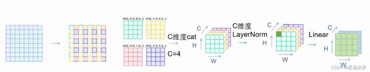
layer = BasicLayer(..., downsample=PatchMerging if (i_layer < self.num_layers - 1) else None, ...)Patch Merging Is used to reduce Block image The resolution of the x0.5, And the number of characteristic channels x2. This is similar to CNN In each block Previous use stride=2 Convolution of / Pool layer to reduce resolution , At the same time, the characteristic channel is doubled .
Realization : In the direction of rows and columns , Take elements every other one ; Spliced into a tensor in the channel dimension ; Then transform the tensor to be used in the channel dimension LayerNorm operation . Finally using nn.Linear Adjust channel dimension .

Code :
class PatchMerging(nn.Module):
    r""" Patch Merging Layer.

    Args:
        input_resolution (tuple[int]): Resolution of input feature.
        dim (int): Number of input channels.
        norm_layer (nn.Module, optional): Normalization layer.  Default: nn.LayerNorm
    """

    def __init__(self, input_resolution, dim, norm_layer=nn.LayerNorm):
        super().__init__()
        self.input_resolution = input_resolution
        self.dim = dim
        self.reduction = nn.Linear(4 * dim, 2 * dim, bias=False)
        self.norm = norm_layer(4 * dim)

    def forward(self, x):
        """
        x: B, H*W, C
        """
        H, W = self.input_resolution
        B, L, C = x.shape
        assert L == H * W, "input feature has wrong size"
        assert H % 2 == 0 and W % 2 == 0, f"x size ({H}*{W}) are not even."

        x = x.view(B, H, W, C)

        x0 = x[:, 0::2, 0::2, :]  # B H/2 W/2 C
        x1 = x[:, 1::2, 0::2, :]  # B H/2 W/2 C
        x2 = x[:, 0::2, 1::2, :]  # B H/2 W/2 C
        x3 = x[:, 1::2, 1::2, :]  # B H/2 W/2 C
        x = torch.cat([x0, x1, x2, x3], -1)  # B H/2 W/2 4*C
        x = x.view(B, -1, 4 * C)  # B H/2*W/2 4*C

        x = self.norm(x)
        x = self.reduction(x)

        return x
4. Image classification task
self.num_features = int(embed_dim * 2 ** (self.num_layers - 1))  # 96 * 2^3 =768
self.norm = nn.LayerNorm(self.num_features)
self.avgpool = nn.AdaptiveAvgPool1d(1)
self.head = nn.Linear(self.num_features, num_classes) if num_classes > 0 else nn.Identity()

x = self.norm(x)  # B L C
x = self.avgpool(x.transpose(1, 2))  # B C 1
x = torch.flatten(x, 1) # B C

x = self.head(x) # B num_classes
for example , Input is (128, 3, 224, 224),BasicLayer_3 The output of the system is (128, 49, 768), In the code C by 96.
(128, 49, 768)  (128, 49, 768)
  (128, 768, 49)
  (128, 768, 1)
  (128, 768)
  (128, num_classes)
5. To be continued
- cyclic shift + reverse cyclic shift
- SW-MSA
- W-MSA and MSA Complexity comparison of
6. Reference resources
The illustration Swin Transformer - You know
Detailed explanation of the paper :Swin Transformer - You know
https://github.com/microsoft/Swin-Transformer
12.1 Swin-Transformer Network structure details _ Bili, Bili _bilibili
边栏推荐
- [successful graduation] [1] - visit [student management information system]
- 新系列单片机还延续了STM32产品家族的低电压和节能两大优势
- PIP references domestic sources
- Project scope management__ Scope management plan and scope specification
- [CSDN] C1 training problem analysis_ Part II_ Web Foundation
- C language enumeration type
- 应用最广泛的8位单片机当然也是初学者们最容易上手学习的单片机
- Comment la base de données mémoire joue - t - elle l'avantage de la mémoire?
- [keil5 debugging] warning:enumerated type mixed with other type
- Successful graduation [3]- blog system update...
猜你喜欢
![[22 graduation season] I'm a graduate yo~](/img/e2/5393b051e2d1cb4c307efdfb3f9148.png)
[22 graduation season] I'm a graduate yo~

51 MCU tmod and timer configuration

在三线城市、在县城,很难毕业就拿到10K
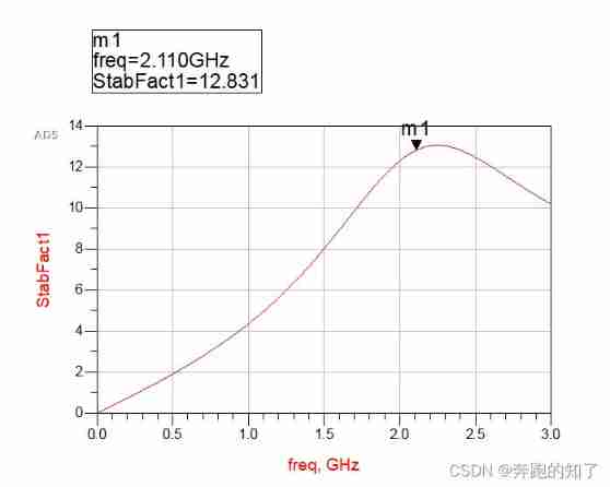
ADS simulation design of class AB RF power amplifier
![[Li Kou brush question notes (II)] special skills, module breakthroughs, classification and summary of 45 classic questions, and refinement in continuous consolidation](/img/06/7fd985faf8806ceface3864d4b3180.png)
[Li Kou brush question notes (II)] special skills, module breakthroughs, classification and summary of 45 classic questions, and refinement in continuous consolidation

Oracle database SQL statement execution plan, statement tracking and optimization instance

03 FastJson 解决循环引用
C language enumeration type

It is difficult to quantify the extent to which a single-chip computer can find a job
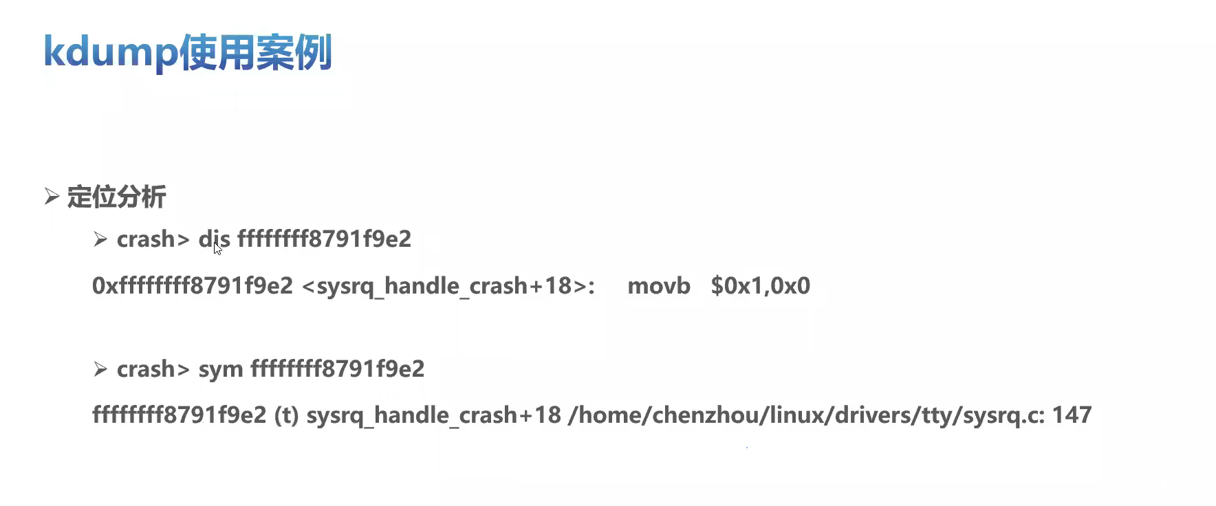
Openeuler kernel technology sharing - Issue 1 - kdump basic principle, use and case introduction

随机推荐
01 business structure of imitation station B project
Vector processor 9_ Basic multilevel interconnection network
Stm32-hal library learning, using cubemx to generate program framework
Programming ideas are more important than anything, not more than who can use several functions, but more than the understanding of the program
Serial communication based on 51 single chip microcomputer
Hal library sets STM32 clock
01 business structure of imitation station B project
JS foundation - prototype prototype chain and macro task / micro task / event mechanism
没有多少人能够最终把自己的兴趣带到大学毕业上
51 MCU tmod and timer configuration
All processes of top ten management in project management
Oracle database SQL statement execution plan, statement tracking and optimization instance
Do you understand automatic packing and unpacking? What is the principle?
Project cost management__ Plan value_ Earned value_ Relationship among actual cost and Countermeasures
JMX、MBean、MXBean、MBeanServer 入门
CEF下载,编译工程
Mobile phones are a kind of MCU, but the hardware it uses is not 51 chip
Stm32 NVIC interrupt priority management
Drive and control program of Dianchuan charging board for charging pile design
Successful graduation [3]- blog system update...