【R】 [density clustering, hierarchical clustering, expectation maximization clustering]

• Data sets ：2 Dimensional datasets —Countries, You can clearly show the clustering effect with a plan . The dataset contains 68 The birth rate of countries and regions （%） And mortality （%）.

• The experiment purpose ： By analyzing the data set , Find the birth rate and mortality rate in different countries and regions , And according to the comparison Prediction and defense of public health .

• This experiment uses Density clustering 、 Hierarchical clustering and expectation maximization clustering The above data sets are Clustering analysis , And the three clustering methods are simply compared .

1． Load the dataset 、 Preprocessing set visualization

1.1 Load data set

setwd(" The path where the dataset is stored ")
countries<-read.csv("countries.csv") # Reading data sets 

1.2 Data preprocessing

dim(countries)
head(countries)

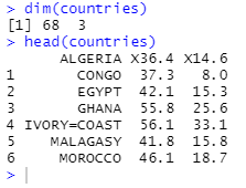
from head() As a result, the data set has no column names , And the row corresponds to a number , Not the corresponding country .

Now we're going to Modify the row and column names ：

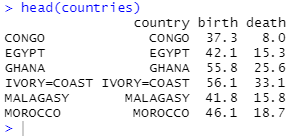
names(countries)<-c("country","birth","death") # Set three variable names 
var<-countries$country # Take variables  country  The value of is assigned to  var

var<-as.character(var) # Change the assigned to character 
head(var)

for(i in 1:68) row.names(countries)[i]=var[i]# Put the dataset  countries  The row name of is named as the response country name 
head(countries)

1.3 Visualize the sample points

plot(countries$birth,countries$death) # Draw all  68  A sample points 
c<-which(countries$country==" Cluster point 1")
d<-which(countries$country==" Cluster point 2")
e<-which(countries$country==" Cluster point 3")
f<-which(countries$country==" Cluster point 4")
g<-which(countries$country==" Cluster point 5")
h<-which(countries$country==" Cluster point 6")
m<-which.max(countries$birth) # Get the position of the highest birth rate in the data set 

points(countries[c(c,d,e,f,g,h,m),-1],pch=16)# Mark the above sample points with solid dots 

legend(countries$birth[c],countries$death[c]," Sirius ",bty="n",xjust=0.5,cex=0.8) 
# The legend marking the sample points in Sirius area 
legend(countries$birth[d],countries$death[d]," Betelgeuse Seven Star area ",bty="n",xjust=0.5,cex=0.8)
legend(countries$birth[e],countries$death[e]," Blue shift area ",bty="n",xjust=0.5,cex=0.8)
legend(countries$birth[f],countries$death[f]," Filipino Star area ",bty="n",xjust=0.5,cex=0.8)
legend(countries$birth[g],countries$death[g]," Cecil sector ",bty="n",xjust=0.5,cex=0.8)
legend(countries$birth[h],countries$death[h]," Arcturus ",bty="n",xjust=0.5,cex=0.8)
legend(countries$birth[m],countries$death[m],countries$country[m],bty="n",xjust=1,cex=0.8)

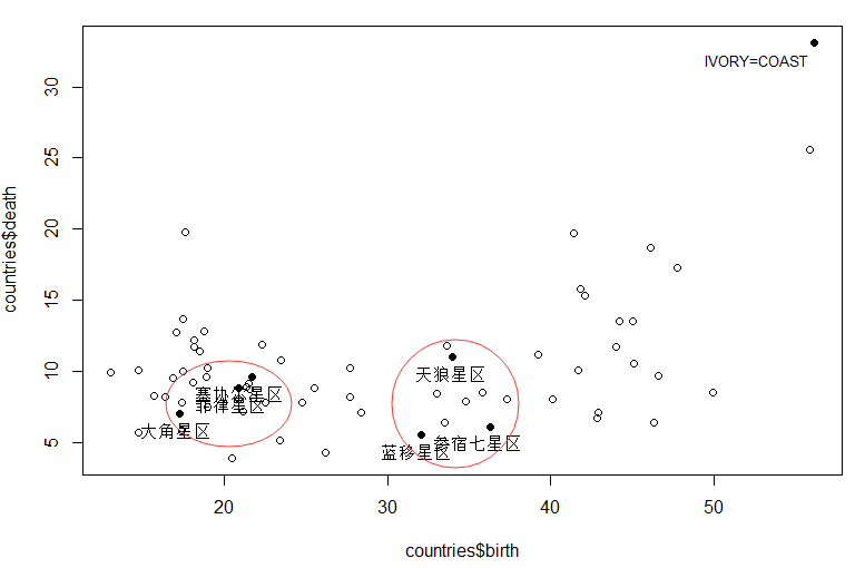
We can probably see from the picture ,( Filipino Star area 、 Cecil sector 、 Arcturus ) Can be grouped into one class ;
9 Sirius 、 Betelgeuse Seven Star area 、 Blue shift area ) For one kind ;
Ivory Coast / Africa (IVORY-COAST) Class I .
also （ Sirius ） And （ Betelgeuse Seven Star area 、 Blue shift area ） The birth rate is similar , The mortality rate is about 5 Percentage .

The above is the data preprocessing part , Let's start clustering the data set density ：

2． Density clustering （DBSCAN Algorithm ）

2.1 Load package

install.packages("fpc")
library(fpc)

2.2 Set clustering parameter threshold and visualize

# Set parameters of clustering ： Radius and density 
ds1=dbscan(countries[,-1],eps=1,MinPts=5)# Take the radius parameter  eps  by  1, Density threshold  MinPts  by  5
ds2=dbscan(countries[,-1],eps=4,MinPts=5)# Take the radius parameter  eps  by  4, Density threshold  MinPts  by  5
ds3=dbscan(countries[,-1],eps=4,MinPts=2)# Take the radius parameter  eps  by  4, Density threshold  MinPts  by  2
ds4=dbscan(countries[,-1],eps=8,MinPts=2)# Take the radius parameter  eps  by  8, Density threshold  MinPts  by  2

ds1;ds2;ds3;ds4

par(mfcol=c(2,2)) # Set up  4  According to  2  That's ok  2  The blank position of the column 
plot(ds1,countries[,-1],main="1:MinPts=5 eps=1")# draw MinPts=5,eps=1  The result of time 
plot(ds3,countries[,-1],main="3:MinPts=2 eps=4")# draw MinPts=2,eps=4  The result of time 
plot(ds2,countries[,-1],main="2:MinPts=5 eps=4")# draw MinPts=5,eps=4  The result of time 
plot(ds4,countries[,-1],main="4:MinPts=2 eps=8")# draw MinPts=2,eps=8  The result of time 

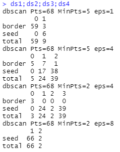
radius 1, threshold 5：DBSCAN The algorithm determines most samples as noise points only 9 Sample points with very similar density are determined as effective clusters .

radius 4, threshold 5： have only 5 Samples are judged as noise points , The remaining samples are classified into the corresponding category clusters .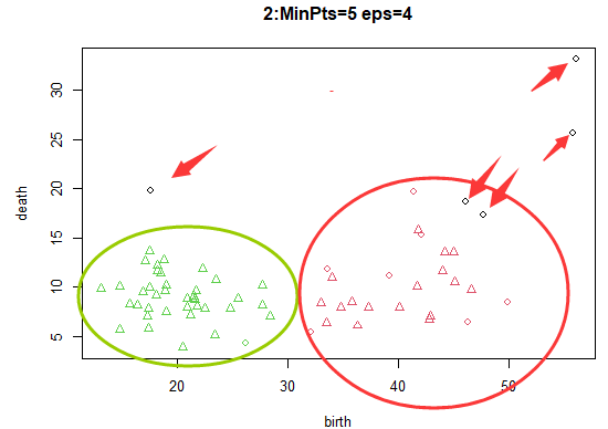

radius 4, threshold 2： More samples are classified into the category of mutually dense samples .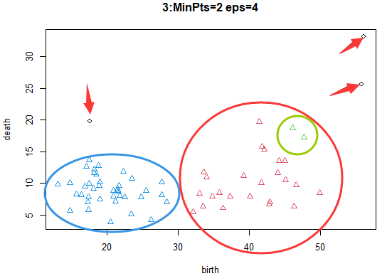

radius 8, threshold 2： Because the core object 、 The determination condition that the density can reach the same height year is relaxed to a great extent , As one can imagine , A large number of sample points will be classified into the same category .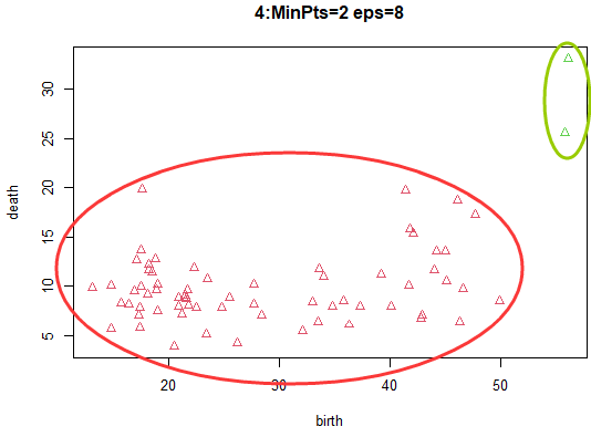

By visualization , obtain DBSCAN The parameter value rule of the algorithm ：

• Radius parameter (eps) And threshold parameters (MinPts) The larger the value difference of , The smaller the total number of categories ;
• Radius parameter (eps) Relative to the threshold parameter (MinPts) More hours , The more samples are judged as noise points or edge points .

2.3 Density clustering

1） Before density clustering, we need to calculate the distance matrix of the data set ：

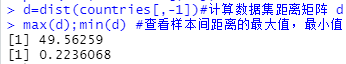
d=dist(countries[,-1])# Calculate the data set distance matrix  d
max(d);min(d) # Check the maximum distance between samples , minimum value 

2） Segment the distance between samples ：
The difference between the maximum value and the minimum value 50 （49.56259-0.2236068） about , Take the number in the middle as 30 And show the data classification results

library(ggplot2) 
interval=cut_interval(d,30) 
# Segment the distance between samples , The difference between the maximum value and the minimum value  50  about , Take the number in the middle as  30
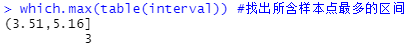
table(interval) # Show the data classification results 

which.max(table(interval)) # Find the interval with the most sample points 

3） With different thresholds 、 Density clustering with different radii and visualization

According to the picture above ： The distance between sample points is mostly (3.15,5.16] Between , So consider Radius parameter (eps) The values for 3、4、5、 The density threshold parameter is 1-10：

for(i in 3:5) # The radius parameter is  3,4,5
{
    
  for(j in 1:10) # The density threshold parameter is  1  to  10
  {
    
    ds=dbscan(countries[,-1],eps=i,MinPts=j) # In the radius of i, The threshold for j when , do dbscan  distance 
    print(ds)
  }
}

Some results are shown above

3． Hierarchical clustering （hclust Algorithm ）

3.1 Hierarchical clustering

fit_hc=hclust(dist(countries[,-1])) # Yes  countries  The data set is subject to pedigree clustering 
print(fit_hc)
plot(fit_hc)

From the cluster diagram （ No label ） You can see , In the picture Each sample point at the bottom occupies a branch and forms its own class , The more you look up, the more sample points under a branch , Until all the sample points at the bottom are grouped into one class . Measure the height of the tree with the height index on the left side of the graph .

3.2 Adjust the hierarchical clustering parameters and display the results

group_k3=cutree(fit_hc,k=3)
# Using pruning function  cutree() Parameters in  k  control input  3  The result of pedigree clustering of categories 
group_k3
table(group_k3)

group_h18=cutree(fit_hc,h=18)
# Using the parameters in the pruning function  h  Control output Height=18  The result of pedigree clustering 
group_h18
table(group_h18)

The above figure shows the use of Parameters in pruning function h Control output Height=3 and 18 Clustering results when .

sapply(unique(group_k3),function(g)countries$country[group_k3==g])
# See above K=3 The clustering results of each category of samples 

plot(fit_hc)
rect.hclust(fit_hc,k=4,border="blue") 
# Frame with a blue rectangle 4 Clustering results of classification 
rect.hclust(fit_hc,k=3,border="red")
# Frame... With a red rectangle 3 Clustering results of classification 
rect.hclust(fit_hc,k=7,which=c(2,6),border="green")
# Frame with a green rectangle 7 The number of categories 2 Class and 6 Clustering results of classes 

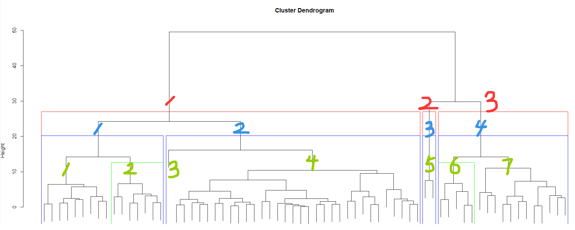
The clustering effect of setting the number of categories is shown in the above figure

4． Expectation maximization clustering （Mclust Algorithm ）

4.1 Expect to maximize clustering and obtain relevant information

1） Load related packages

library(mclust)

2） Perform expectation maximization clustering and obtain relevant information

fit_EM=Mclust(countries[,-1]) # Yes  countries  The dataset goes on  EM  clustering 
summary(fit_EM)# obtain  EM  Information summary of clustering results 
summary(fit_EM,parameters=TRUE) # obtain  EM  Details of clustering results 

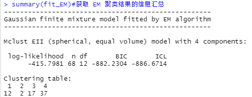
It can be seen from the results , The optimal number of categories is 4, And each category contains 12、2、17、37 Samples .

4.2 Graphic display of results

plot(fit_EM)

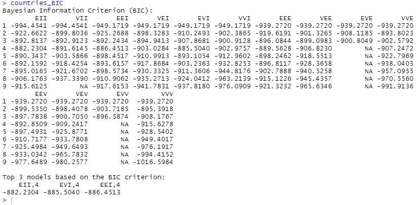
countries_BIC<-mclustBIC(countries[,-1])# Get data set  countries  Under the number of models and categories  BIC  value 
countries_BICsum=summary(countries_BIC,data=countries[,-1])# Get data set  countries  Of  BIC  Value overview 
countries_BICsum

countries_BIC
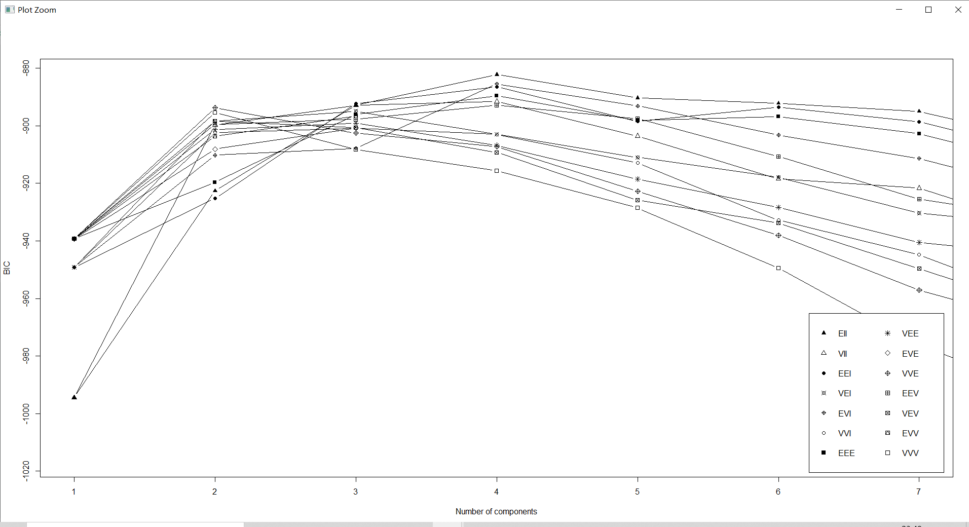
plot(countries_BIC,G=1:7,col="black")
names(countries_BICsum)

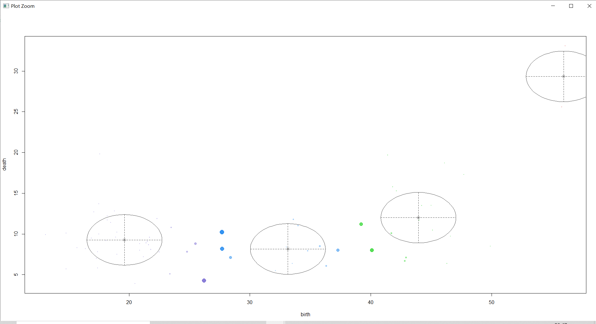
mclust2Dplot(countries[,-1],classification=countries_BICsum$classification,parameters=countries_BICsum$parameters,col="black")
# Draw a classification map 

① see BIC：

② see classification：

③ see uncertainty：

④ see density：

countries_BIC<-mclustBIC(countries[,-1])# Get data set  countries  Under the number of models and categories  BIC  value 
countries_BICsum=summary(countries_BIC,data=countries[,-1])# Get data set  countries  Of  BIC  Value overview 
countries_BICsum
countries_BIC

plot(countries_BIC,G=1:7,col="black")
names(countries_BICsum)

mclust2Dplot(countries[,-1],classification=countries_BICsum$classification,parameters=countries_BICsum$parameters,col="black")
# Draw a classification map 

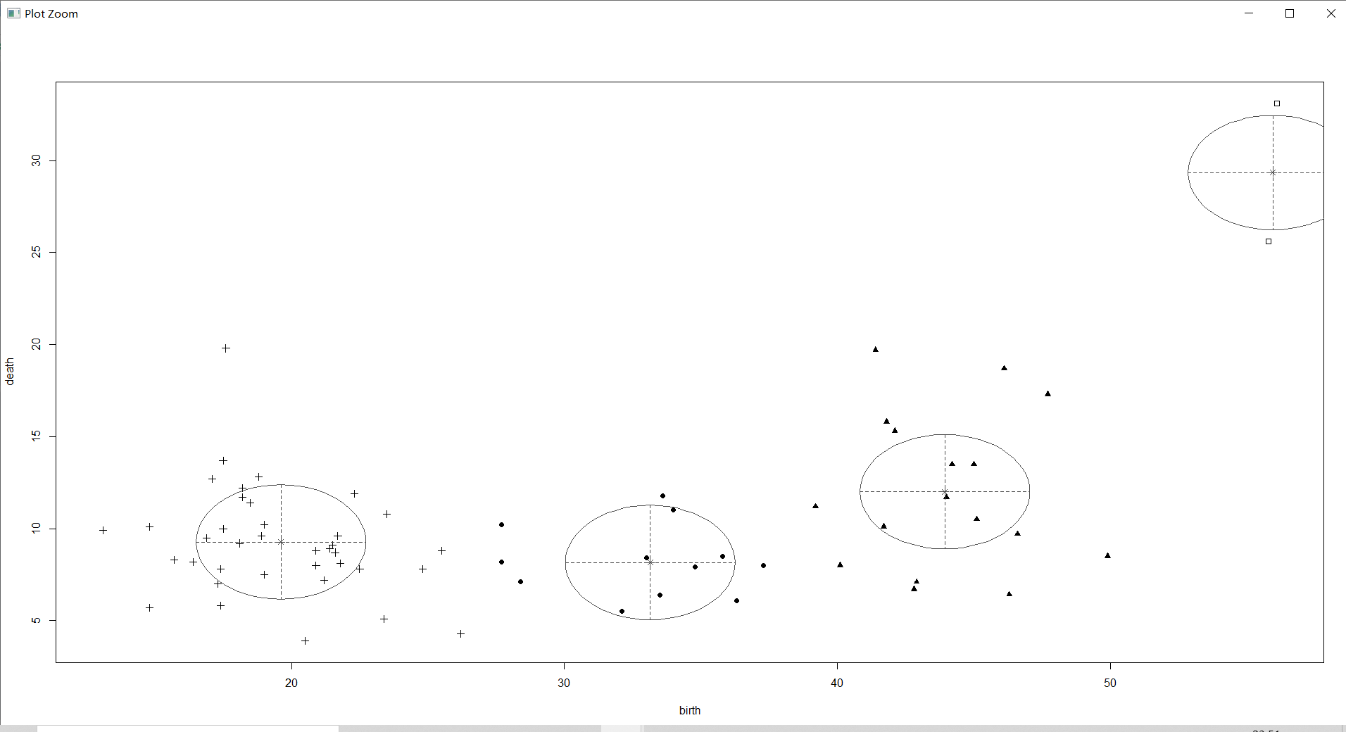
The above figure not only circles the main distribution areas of each category of samples with ellipses , The center point of the category is marked , And the probability that the sample belongs to the corresponding category is displayed by the size of the sample point graph .

countries_Dens=densityMclust(countries[,-1])# Estimate the density of each sample 

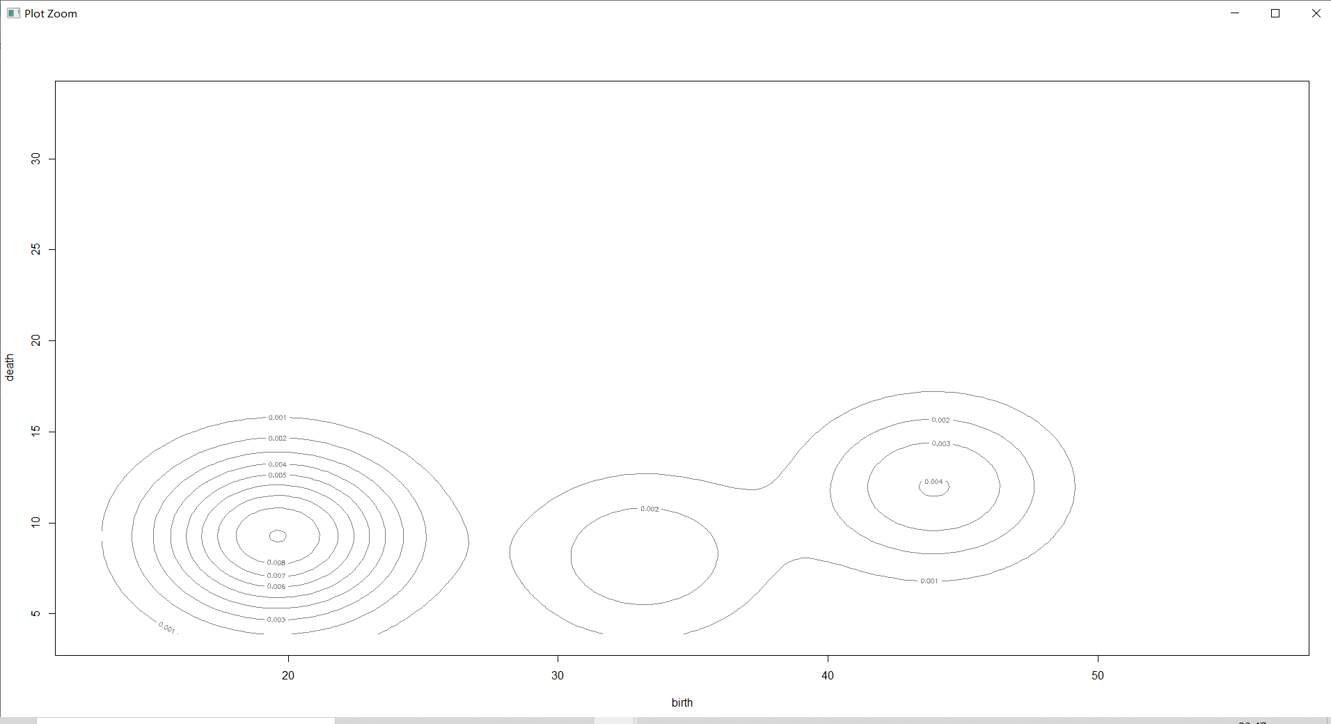
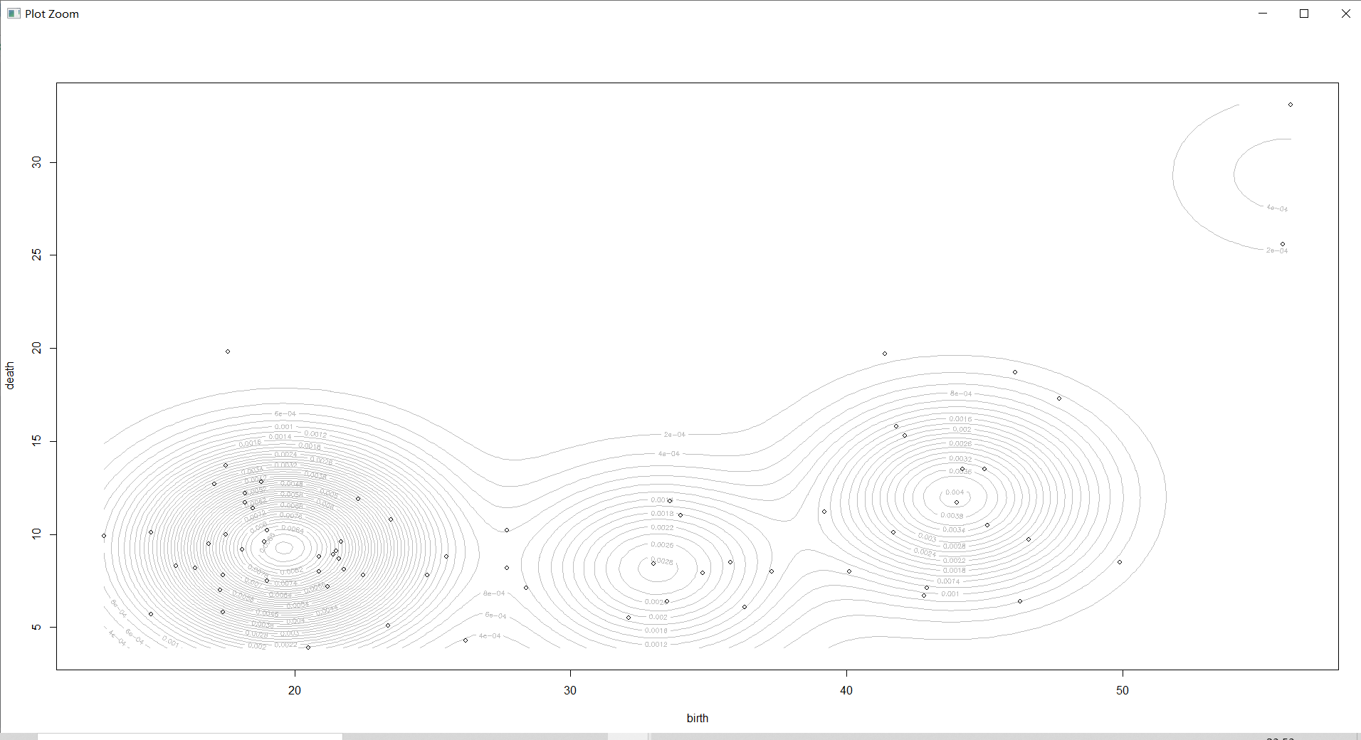
2 Dimensional density diagram

plot(countries_Dens,countries[,-1],col="grey",nlevels=55)# do  2  Dimensional density diagram 

① see BIC：

② see density：

3 Dimensional density diagram

plot(countries_Dens,type="persp",col=grey(0.8)) # do  3  Dimensional density diagram 

① see BIC：

② see density：

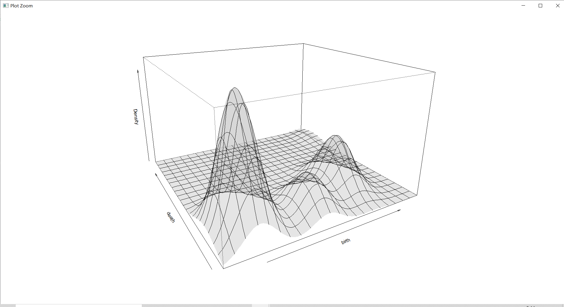
（ Need to load for a while ）

Density estimation diagram is a three-dimensional graph , It shows the density area more intuitively , Make a general understanding of the density .

summary

Pedigree clustering ？： From the visualization, we can feel the difference between pedigree clustering and mean clustering and central point clustering in the previous experiment . The visual graph of genealogical clustering is like a genealogy, which is divided into many different branches , The bottom of the branch is the name of all sample points .

Density clustering ： The difference from other clusters is You need to set the threshold and radius . Relative to the above mean clustering 、 For central point clustering and pedigree clustering , Its advantage is to make up for the former can only find “ Class round ” The defects of clustering , The density clustering algorithm is based on “ density ” To cluster , Clusters of arbitrary shape can be found in spatial databases with noise .

Expectation maximization clustering ： The idea is very clever , When using this algorithm for clustering , it Treat the data set as a probability model with hidden variables , And to achieve model optimization , That is, the purpose is to obtain the clustering method that is most consistent with the nature of the data , adopt “ Repeatedly estimate ” Model parameters to find the optimal solution , At the same time, the corresponding optimal number of categories is given K. therefore , Expect to maximize clustering relative to the previously mentioned clustering More abstract .

Reference

dbscan: Density-based Spatial Clustering of Applications with Noise (DBSCAN)/ writing RDocumentation

hclust: Hierarchical Clustering/ writing RDocumentation

Mclust: Model-Based Clustering/ writing RDocumentation

DBSCAN/ Baidu Encyclopedia

DBSCAN Algorithm / Wen Jianshu @dreampai

Summary of clustering analysis algorithm / Wen Zhihu @ Shi Xian

be based on EM Clustering algorithm R package mclust/ Wen Jianshu @ Xiaorunze

R Language data mining practice ---- Common functions of cluster analysis / Wen personal library @ new user 26922hFh

Experimental data

Data sets &R The language code
Extraction code ：1111（ Here should be automatically filled ）