Software package for optimization scientific research field

Software package for optimizing scientific research field

Project introduction

  optimtool It adopts the 《 optimization ： modeling 、 Algorithm and theory 》 Some of the theoretical and methodological frameworks in this book , Use of the Numpy Packet efficient processing of inter array operations, etc , Cleverly applied Sympy Internally supported .jacobian Other methods , And combine Python Built in functions dict And zip Realized Sympy Matrix to Numpy Matrix transformation , Finally, we designed a system for optimization research Python tool kit . Researchers can simply pip Command to download and use . The algorithms of unconstrained optimization and constrained optimization in the project still need to be updated 、 Maintenance and expansion , And the algorithm applied to mixed constraint optimization will be launched in the future . We welcome people who love mathematics 、 Programmers from all walks of life join the team of developing and updating optimization calculation methods , Propose a new framework or algorithm , Become a member of the milestone .

Project structure

|- optimtool
    |-- constrain
        |-- __init__.py
        |-- equal.py
        |-- mixequal.py
        |-- unequal.py
    |-- example
        |-- __init__.py
        |-- Lasso.py
        |-- WanYuan.py
    |-- functions
        |-- __init__.py
        |-- linear_search.py
        |-- tools.py
    |-- hybrid
        |-- __init__.py
        |-- approximate_point_gradient.py
    |-- unconstrain
        |-- __init__.py
        |-- gradient_descent.py
        |-- newton.py
        |-- newton_quasi.py
        |-- nonlinear_least_square.py
        |-- trust_region.py  
    |-- __init__.py 

   Because when solving the global or local convergence points of different objective functions , Different methods for finding the convergence point will have different convergence efficiency and different application scope , And in the process of research, research methods in different fields have been constantly put forward 、 modify 、 perfect 、 expand , So these methods have become popular nowadays Optimization method . All internally supported algorithms in this project , It's all in the norm 、 derivative 、 convex set 、 Convex function 、 Conjugate functions 、 It is designed and perfected on the basis of basic methodology such as subgradient and optimization theory .

  optimtool Built in things like Barzilar Borwein Nonmonotonic gradient descent method 、 Modified Newton's method 、 Limited memory BFGS Method 、 Truncated conjugate gradient method - Trust region method 、 gaussian - Newton method and other unconstrained optimization algorithms with good convergence efficiency and properties , And the quadratic penalty function method for solving constrained optimization problems 、 Augmented Lagrangian method and other algorithms .

Github Source code ：linjing-lab/optimtool

Start using

Unconstrained optimization algorithm （unconstrain）

import optimtool.unconstrain as ou
ou.[ Method name ].[ Function name ]([ Objective function ], [ Parameter table ], [ Initial iteration point ])

Gradient descent method （gradient_descent）

ou.gradient_descent.[ Function name ]([ Objective function ], [ Parameter table ], [ Initial iteration point ])

Method head	explain
solve(funcs, args, x_0, draw=True, output_f=False, epsilon=1e-10, k=0)	The exact step size is solved by solving the equation
steepest(funcs, args, x_0, draw=True, output_f=False, method=“wolfe”, epsilon=1e-10, k=0)	Use the line search method to solve the inexact step size （ By default wolfe Line search ）
barzilar_borwein(funcs, args, x_0, draw=True, output_f=False, method=“grippo”, M=20, c1=0.6, beta=0.6, alpha=1, epsilon=1e-10, k=0)	Use Grippo And Zhang hanger The proposed nonmonotonic line search method updates the step size

Newton method （newton)

ou.newton.[ Function name ]([ Objective function ], [ Parameter table ], [ Initial iteration point ])

Method head	explain
classic(funcs, args, x_0, draw=True, output_f=False, epsilon=1e-10, k=0)	By directly calculating the second derivative matrix of the objective function （ Heather matrix ） Perform inversion to obtain the step size of the next step
modified(funcs, args, x_0, draw=True, output_f=False, method=“wolfe”, m=20, epsilon=1e-10, k=0)	Modify the current Hessian matrix to ensure its positive definiteness （ At present, only one correction method is connected ）
CG(funcs, args, x_0, draw=True, output_f=False, method=“wolfe”, epsilon=1e-6, k=0)	Adopt Newton - The conjugate gradient method is used to solve the gradient （ A kind of inexact Newton method ）

Quasi Newton method （newton_quasi）

ou.newton_quasi.[ Function name ]([ Objective function ], [ Parameter table ], [ Initial iteration point ])

Method head	explain
bfgs(funcs, args, x_0, draw=True, output_f=False, method=“wolfe”, m=20, epsilon=1e-10, k=0)	BFGS Method to update the Hessian matrix
dfp(funcs, args, x_0, draw=True, output_f=False, method=“wolfe”, m=20, epsilon=1e-4, k=0)	DFP Method to update the Hessian matrix
L_BFGS(funcs, args, x_0, draw=True, output_f=False, method=“wolfe”, m=6, epsilon=1e-10, k=0)	Double loop method update BFGS Heather matrix

Nonlinear least square method （nonlinear_least_square）

ou.nonlinear_least_square.[ Function name ]([ Objective function ], [ Parameter table ], [ Initial iteration point ])

Method head	explain
gauss_newton(funcr, args, x_0, draw=True, output_f=False, method=“wolfe”, epsilon=1e-10, k=0)	gaussian - Newton's method framework , Include OR Decomposition and other operations
levenberg_marquardt(funcr, args, x_0, draw=True, output_f=False, m=100, lamk=1, eta=0.2, p1=0.4, p2=0.9, gamma1=0.7, gamma2=1.3, epsilon=1e-10, k=0)	Levenberg Marquardt Proposed methodology framework

Trust region method （trust_region）

ou.trust_region.[ Function name ]([ Objective function ], [ Parameter table ], [ Initial iteration point ])

Method head	explain
steihaug_CG(funcs, args, x_0, draw=True, output_f=False, m=100, r0=1, rmax=2, eta=0.2, p1=0.4, p2=0.6, gamma1=0.5, gamma2=1.5, epsilon=1e-6, k=0)	Truncated conjugate gradient method is used to search step size in this method

Constrained optimization algorithm （constrain）

import optimtool.constrain as oc
oc.[ Method name ].[ Function name ]([ Objective function ], [ Parameter table ], [ Equality constraint table ], [ Inequality divisor table ], [ Initial iteration point ])

Equality constraints （equal）

oc.equal.[ Function name ]([ Objective function ], [ Parameter table ], [ Equality constraint table ], [ Initial iteration point ])

Method head	explain
penalty_quadratic(funcs, args, cons, x_0, draw=True, output_f=False, method=“gradient_descent”, sigma=10, p=2, epsilon=1e-4, k=0)	Add a second penalty
lagrange_augmented(funcs, args, cons, x_0, draw=True, output_f=False, method=“gradient_descent”, lamk=6, sigma=10, p=2, etak=1e-4, epsilon=1e-6, k=0)	Augmented Lagrange multiplier method

Inequality constraints （unequal）

oc.unequal.[ Function name ]([ Objective function ], [ Parameter table ], [ Inequality constraint table ], [ Initial iteration point ])

Method head	explain
penalty_quadratic(funcs, args, cons, x_0, draw=True, output_f=False, method=“gradient_descent”, sigma=10, p=0.4, epsilon=1e-10, k=0)	Add a second penalty
penalty_interior_fraction(funcs, args, cons, x_0, draw=True, output_f=False, method=“gradient_descent”, sigma=12, p=0.6, epsilon=1e-6, k=0)	Add penalty term of fractional function
penalty_interior_log(funcs, args, cons, x_0, draw=True, output_f=False, sigma=12, p=0.6, epsilon=1e-10, k=0)	An approximate point gradient method is added to solve the problem of iteration point overflow
lagrange_augmented(funcs, args, cons, x_0, draw=True, output_f=False, method=“gradient_descent”, muk=10, sigma=8, alpha=0.2, beta=0.7, p=2, eta=1e-1, epsilon=1e-4, k=0)	Augmented Lagrange multiplier method

Mixed equality constraints （mixequal）

oc.mixequal.[ Function name ]([ Objective function ], [ Parameter table ], [ Equality constraint table ], [ Inequality constraint table ], [ Initial iteration point ])

Method head	explain
penalty_quadratic(funcs, args, cons_equal, cons_unequal, x_0, draw=True, output_f=False, method=“gradient_descent”, sigma=10, p=0.6, epsilon=1e-10, k=0)	Add a second penalty
penalty_L1(funcs, args, cons_equal, cons_unequal, x_0, draw=True, output_f=False, method=“gradient_descent”, sigma=1, p=0.6, epsilon=1e-10, k=0)	L1 Exact penalty function method
lagrange_augmented(funcs, args, cons_equal, cons_unequal, x_0, draw=True, output_f=False, method=“gradient_descent”, lamk=6, muk=10, sigma=8, alpha=0.5, beta=0.7, p=2, eta=1e-3, epsilon=1e-4, k=0)	Augmented Lagrange multiplier method

Hybrid optimization algorithm （hybrid）

import optimtool.hybrid as oh

Approximate point gradient descent method （approximate_point_gradient）

oh.approximate_point_gradient.[ Adjacent operator name ]([ Differentiable functions ], [ coefficient ], [ function 2], [ Parameter table ], [ Initial iteration point ])

Method head	explain
L1(funcs, mu, gfun, args, x_0, draw=True, output_f=False, t=0.01, epsilon=1e-6, k=0)	L1 Norm adjacency operator
neg_log(funcs, mu, gfun, args, x_0, draw=True, output_f=False, t=0.01, epsilon=1e-6, k=0)	Negative logarithmic proximity operator

Application of methods （example）

import optimtool.example as oe

Lasso problem （Lasso）

oe.Lasso.[ Function name ]([ matrix A], [ matrix b], [ factor mu], [ Parameter table ], [ Initial iteration point ])

Method head	explain
gradient_descent(A, b, mu, args, x_0, draw=True, output_f=False, delta=10, alp=1e-3, epsilon=1e-2, k=0)	Smooth Lasso Function method
subgradient(A, b, mu, args, x_0, draw=True, output_f=False, alphak=2e-2, epsilon=1e-3, k=0)	The subgradient method Lasso Avoid first-order non derivative
penalty(A, b, mu, args, x_0, draw=True, output_f=False, gamma=0.1, epsilon=1e-6, k=0)	Penalty function method
approximate_point_gradient(A, b, mu, args, x_0, draw=True, output_f=False, epsilon=1e-6, k=0)	Neighborhood operator update

The problem of curve tangency （WanYuan）

oe.WanYuan.[ Function name ]([ The slope of the line ], [ Intercept of line ], [ Coefficient of quadratic term ], [ Coefficient of first-order term ], [ Constant term ], [ The abscissa of the center of the circle ], [ The ordinate of the center of the circle ], [ Initial iteration point ])

Problem description ：

 The slope and intercept of a given line , Given the quadratic coefficient of a parabolic function , First order coefficient and constant term .  It is required to solve a circle with a given center , The circle is simultaneously connected with the parabola 、 Tangent line , If there is a feasible solution , Please give the coordinates of the tangent point .

Method head	explain
gauss_newton(m, n, a, b, c, x3, y3, x_0, draw=False, eps=1e-10)	Use Gauss - Newton's method is used to solve the constructed 7 A residual function

Test cases

Unconstrained optimization problem testing

import sympy as sp
import matplotlib.pyplot as plt
import optimtool as oo

f, x1, x2, x3, x4 = sp.symbols("f x1 x2 x3 x4")
f = (x1 - 1)**2 + (x2 - 1)**2 + (x3 - 1)**2 + (x1**2 + x2**2 + x3**2 + x4**2 - 0.25)**2
funcs = f # [f] \ (f) \ sp.Matrix([f])
args = [x1, x2, x3, x4] # (x1, x2, x3, x4) \ sp.Matrix([args])
x_0 = (1, 2, 3, 4)

f_list = []
title = ["gradient_descent_barzilar_borwein", "newton_CG", "newton_quasi_L_BFGS", "trust_region_steihaug_CG"]
colorlist = ["maroon", "teal", "slateblue", "orange"]
_, _, f = oo.unconstrain.gradient_descent.barzilar_borwein(funcs, args, x_0, False, True)
f_list.append(f)
_, _, f = oo.unconstrain.newton.CG(funcs, args, x_0, False, True)
f_list.append(f)
_, _, f = oo.unconstrain.newton_quasi.L_BFGS(funcs, args, x_0, False, True)
f_list.append(f)
_, _, f = oo.unconstrain.trust_region.steihaug_CG(funcs, args, x_0, False, True)
f_list.append(f)

# draw
handle = []
for j, z in zip(colorlist, f_list):
    ln, = plt.plot([i for i in range(len(z))], z, c=j, marker='o', linestyle='dashed')
    handle.append(ln)
plt.xlabel("$Iteration \ times \ (k)$")
plt.ylabel("$Objective \ function \ value: \ f(x_k)$")
plt.legend(handle, title)
plt.title("Performance Comparison")
plt.show()

Nonlinear least square problem testing

import sympy as sp
import matplotlib.pyplot as plt
import optimtool as oo

r1, r2, x1, x2 = sp.symbols("r1 r2 x1 x2")
r1 = x1**3 - 2*x2**2 - 1
r2 = 2*x1 + x2 - 2
funcr = [r1, r2] # (r1, r2) \ sp.Matrix([funcr])
args = [x1, x2] # (x1, x2) \ sp.Matrix([args])
x_0 = (2, 2)

f_list = []
title = ["gauss_newton", "levenberg_marquardt"]
colorlist = ["maroon", "teal"]
_, _, f = oo.unconstrain.nonlinear_least_square.gauss_newton(funcr, args, x_0, False, True)
f_list.append(f)
_, _, f = oo.unconstrain.nonlinear_least_square.levenberg_marquardt(funcr, args, x_0, False, True)
f_list.append(f)

# draw
handle = []
for j, z in zip(colorlist, f_list):
    ln, = plt.plot([i for i in range(len(z))], z, c=j, marker='o', linestyle='dashed')
    handle.append(ln)
plt.xlabel("$Iteration \ times \ (k)$")
plt.ylabel("$Objective \ function \ value: \ f(x_k)$")
plt.legend(handle, title)
plt.title("Performance Comparison")
plt.show()

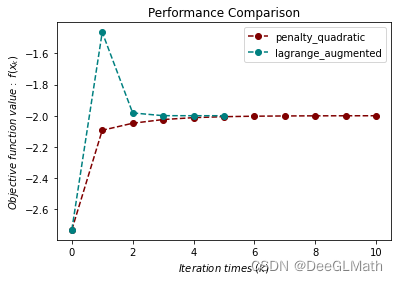
Equality constrained optimization problem testing

import numpy as np
import sympy as sp
import matplotlib.pyplot as plt
import optimtool as oo

f, x1, x2 = sp.symbols("f x1 x2")
f = x1 + np.sqrt(3) * x2
c1 = x1**2 + x2**2 - 1
funcs = f # [f] \ (f) \ sp.Matrix([f])
cons = [c1] # c1 \ (c1) \ sp.Matrix([cons])
args = [x1, x2] # (x1, x2) \ sp.Matrix([args])
x_0 = (-1, -1)

f_list = []
title = ["penalty_quadratic", "lagrange_augmented"]
colorlist = ["maroon", "teal"]
_, _, f = oo.constrain.equal.penalty_quadratic(funcs, args, cons, x_0, False, True)
f_list.append(f)
_, _, f = oo.constrain.equal.lagrange_augmented(funcs, args, cons, x_0, False, True)
f_list.append(f)

# draw
handle = []
for j, z in zip(colorlist, f_list):
    ln, = plt.plot([i for i in range(len(z))], z, c=j, marker='o', linestyle='dashed')
    handle.append(ln)
plt.xlabel("$Iteration \ times \ (k)$")
plt.ylabel("$Objective \ function \ value: \ f(x_k)$")
plt.legend(handle, title)
plt.title("Performance Comparison")
plt.show()

Inequality constrained optimization problem testing

import sympy as sp
import matplotlib.pyplot as plt
import optimtool as oo

f, x1, x2 = sp.symbols("f x1 x2")
f = x1**2 + (x2 - 2)**2
c1 = 1 - x1
c2 = 2 - x2
funcs = f # [f] \ (f) \ sp.Matrix([f])
cons = [c1, c2] # (c1, c2) \ sp.Matrix([cons])
args = [x1, x2] # (x1, x2) \ sp.Matrix([args])
x_0 = (2, 3)

f_list = []
title = ["penalty_quadratic", "penalty_interior_fraction"]
colorlist = ["maroon", "teal"]
_, _, f = oo.constrain.unequal.penalty_quadratic(funcs, args, cons, x_0, False, True, method="newton", sigma=10, epsilon=1e-6)
f_list.append(f)
_, _, f = oo.constrain.unequal.penalty_interior_fraction(funcs, args, cons, x_0, False, True, method="newton")
f_list.append(f)

# draw
handle = []
for j, z in zip(colorlist, f_list):
    ln, = plt.plot([i for i in range(len(z))], z, c=j, marker='o', linestyle='dashed')
    handle.append(ln)
plt.xlabel("$Iteration \ times \ (k)$")
plt.ylabel("$Objective \ function \ value: \ f(x_k)$")
plt.legend(handle, title)
plt.title("Performance Comparison")
plt.show()

Mixed equality constrained optimization problem testing

import sympy as sp
import matplotlib.pyplot as plt
import optimtool as oo

f, x1, x2 = sp.symbols("f x1 x2")
f = (x1 - 2)**2 + (x2 - 1)**2
c1 = x1 - 2*x2
c2 = 0.25*x1**2 - x2**2 - 1
funcs = f # [f] \ (f) \ sp.Matrix([f])
cons_equal = c1 # [c1] \ (c1) \ sp.Matrix([c1])
cons_unequal = c2 # [c2] \ (c2) \ sp.Matrix([c2])
args = [x1, x2] # (x1, x2) \ sp.Matrix([args])
x_0 = (0.5, 1)

f_list = []
title = ["penalty_quadratic", "penalty_L1", "lagrange_augmented"]
colorlist = ["maroon", "teal", "orange"]
_, _, f = oo.constrain.mixequal.penalty_quadratic(funcs, args, cons_equal, cons_unequal, x_0, False, True)
f_list.append(f)
_, _, f = oo.constrain.mixequal.penalty_L1(funcs, args, cons_equal, cons_unequal, x_0, False, True)
f_list.append(f)
_, _, f = oo.constrain.mixequal.lagrange_augmented(funcs, args, cons_equal, cons_unequal, x_0, False, True)
f_list.append(f)

# draw
handle = []
for j, z in zip(colorlist, f_list):
    ln, = plt.plot([i for i in range(len(z))], z, c=j, marker='o', linestyle='dashed')
    handle.append(ln)
plt.xlabel("$Iteration \ times \ (k)$")
plt.ylabel("$Objective \ function \ value: \ f(x_k)$")
plt.legend(handle, title)
plt.title("Performance Comparison")
plt.show()

Lasso Problem testing

import numpy as np
import sympy as sp
import matplotlib.pyplot as plt
import optimtool as oo

import scipy.sparse as ss
f, A, b, mu = sp.symbols("f A b mu")
x = sp.symbols('x1:9')
m = 4
n = 8
u = (ss.rand(n, 1, 0.1)).toarray()
A = np.random.randn(m, n)
b = A.dot(u)
mu = 1e-2
args = x # list(x) \ sp.Matrix(x)
x_0 = tuple([1 for i in range(8)])

f_list = []
title = ["gradient_descent", "subgradient"]
colorlist = ["maroon", "teal"]
_, _, f = oo.example.Lasso.gradient_descent(A, b, mu, args, x_0, False, True, epsilon=1e-4)
f_list.append(f)
_, _, f = oo.example.Lasso.subgradient(A, b, mu, args, x_0, False, True)
f_list.append(f)

# draw
handle = []
for j, z in zip(colorlist, f_list):
    ln, = plt.plot([i for i in range(len(z))], z, c=j, marker='o', linestyle='dashed')
    handle.append(ln)
plt.xlabel("$Iteration \ times \ (k)$")
plt.ylabel("$Objective \ function \ value: \ f(x_k)$")
plt.legend(handle, title)
plt.title("Performance Comparison")
plt.show()

Curve tangent problem test

# import packages
import sympy as sp
import matplotlib.pyplot as plt
import optimtool as oo

# make data
m = 1
n = 2
a = 0.2
b = -1.4
c = 2.2
x3 = 2*(1/2)
y3 = 0
x_0 = (0, -1, -2.5, -0.5, 2.5, -0.05)

# train
oo.example.WanYuan.gauss_newton(1, 2, 0.2, -1.4, 2.2, 2**(1/2), 0, (0, -1, -2.5, -0.5, 2.5, -0.05), draw=True)