【GAN】SAGAN ICML‘19

《Self-Attention Generative Adversarial Networks》ICML’19,Goodfellow A signature .

The deep convolution network can improve GANs Details of generating high resolution pictures . This article aims to solve the problem of generating large-scale correlation （Long-range dependency） The picture area of ,CNN The influence of local receptive field , So in DCGAN On the basis of the introduction of Self-attention.

What problem to solve

When generating, for example, face images , Details are very important , Like left and right eyes , As long as there is a little asymmetry between the left and right eyes , The generated face will be especially unreal , So the area of the left and right eyes is “ Large scale correlation ”（Long-range dependency） Of . There is Long-range dependency There are a lot of , But because of CNN Limitation of local receptive field （ Convolution kernel is difficult to cover a large area ）, It's hard to capture global information , For example, the influence of the left eye on the right eye cannot be seen when convoluting the right eye area , The left and right eyes of the generated face image may not be related .

Want to see the overall information , There are several ways ：1、 Increase the size of convolution kernel 、 Expand the feeling field —— Increase the amount of parameters and calculation , And unless the convolution kernel is as large as the picture , Otherwise, there is still a blind spot in the field of vision ;2、 Deepen the convolution layer —— Increase the amount of calculation ;3、 Use the full connection layer to obtain global information —— lose a great deal through trying to save a little .

So the self- attention Introduction is a simple and efficient method .

How do you do it? ——SAGAN Model

Let's start by introducing ：

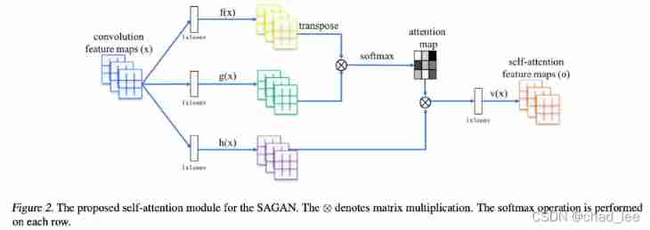
After convolution operation feature map $x$,$\mathbf{x}\in {\mathbb{R}}^{C\times N}$.$f(x),g(x),h(x)$ All are $1\times 1$ Convolution of , take $f(x)$ Transpose and... Of output $g(x)$ Multiply the output of , after softmax Normalize to get a attention map; What will be obtained attention map and $h(x)$ Point by point multiplication , obtain self-attention Characteristic graph .

Concrete realization ：$\mathbf{f}(\mathbf{x})={\mathbf{W}}_{\mathbf{f}}\mathbf{x},\mathbf{g}(\mathbf{x})={\mathbf{W}}_{\mathbf{g}}\mathbf{x},\mathbf{h}(\mathbf{x})={\mathbf{W}}_{\mathbf{h}}\mathbf{x}$,$W_{g} \in R^{\bar{C} \times C}, $$W_f\in R^{\bar{c}\times C},$$W_{h} \in R^{C \times C}$ Is the weight matrix of learning , adopt $1\times 1$ The realization of convolution ,$C$ Number of channels , Used in experiments $\bar{C}=\mathrm{C}/8$.

use ${\beta }_{j,i}$ Indicates that in the synthesis of $j$ When the model is divided into regions, it is right for the $i$ The degree of influence of each location , Yes ：
$${\beta }_{j,i}=\frac{\exp \left(s_{ij}\right)}{{\sum }_{i=1}^N\exp \left(s_{ij}\right)},\text{ where }{s}_{ij}=\mathbf{f}{\left({\mathbf{x}}_{\mathbf{i}}\right)}^T\mathbf{g}\left({\mathbf{x}}_{\mathbf{j}}\right)$$
Output of the final attention layer $\mathbf{o}=\left({\mathbf{o}}_1,{\mathbf{o}}_2,\dots ,{\mathbf{o}}_{\mathbf{j}},\dots ,{\mathbf{o}}_{\mathbf{N}}\right)\in {\mathbb{R}}^{C\times N}$：
$${\mathbf{o}}_{\mathbf{j}}=\mathbf{v}\left(\sum _{i=1}^N{\beta }_{j,i}\mathbf{h}\left({\mathbf{x}}_{\mathbf{i}}\right)\right),\mathbf{h}\left({\mathbf{x}}_{\mathbf{i}}\right)={\mathbf{W}}_{\mathbf{h}}{\mathbf{x}}_{\mathbf{i}},\mathbf{v}\left({\mathbf{x}}_{\mathbf{i}}\right)={\mathbf{W}}_{\mathbf{v}}{\mathbf{x}}_{\mathbf{i}}$$
In addition, residual connection is required ：
$${\mathbf{y}}_{\mathbf{i}}=\gamma {\mathbf{o}}_{\mathbf{i}}+{\mathbf{x}}_{\mathbf{i}}$$
among $\gamma$ Is a learnable proportional parameter ,$\gamma$ Is initialized to 0, Then gradually learn to assign more weights to nonlocal features . The author believes that the early stage mainly depends on CNN Learn local features , The task ranges from simple to difficult , Gradually add weight to nonlocal features . stay SAGAN There are attention modules in the generator and the discriminator . Cross training $D$ and $G$ Of loss：
$$\begin{array}{rl}{L}_D=& -{\mathbb{E}}_{(x,y)\sim p_{data}}[\min (0,-1+D(x,y))]\\ & -{\mathbb{E}}_{z\sim p_z,y\sim p_{\text{data }}}[\min (0,-1-D(G(z),y))]\\ L_G=& -{\mathbb{E}}_{z\sim p_z,y\sim p_{\text{data }}}D(G(z),y)\end{array}$$

From another perspective —— Stacking model

SAGAN It's all about DCGAN Two layers are added on the basis of self-attention layer , Most of the author's open source code also comes from DCGAN, Other open source SAGAN Just add two layers of attention .

This can also be seen from the model diagram in the paper ,$f(x)$ Namely $query$,$g(x)$ Namely $key$,$h(x)$ Namely $value$. The model diagram is just a description of attention Calculation process ：

Stability training GAN The technique of

Spectral Normalization

SAGAN quote SNGAN Spectral norm normalization method , But at the same time D and G Spectral norm normalization is added , Give Way D To satisfy the 1-lipschitz Limit , It also avoids G Too many parameters of lead to abnormal gradient , Make the whole training smooth and efficient .

Normalization of spectral norm is achieved by dividing the gradient by a spectral norm , The spectral norm is derived from the gradient matrix itself .

Two Time- Scale Update Rule(TTUR)

Optimizing G When , We assume by default that our D The discrimination ability is better than the current G The ability to generate is better , such D Talent coaching G Learn for the better . The usual practice is to update D One or more times , Then update G Parameters of ,TTUR A simpler update strategy is proposed , That is to say D and G Set different learning rates , Give Way D Faster convergence . That is, the learning rate of the discriminator is generally set to be greater than that of the generator .

What effect does it bring

In addition to better experimental results , The author also proved that Long-range dependency, Success justifies itself .

visualization attention map：

The arrow represents the dot “query location”, It can be seen that the neural network learns to allocate attention according to the similarity of color and texture , Not just spatial adjacency （ Such as the upper left corner ）, So although some query points are very close in space , But their attention maps can be very different .