当前位置:网站首页>OpenCV Learning notes iii
OpenCV Learning notes iii
2022-06-26 08:26:00 【Cloudy To Sunny.】
opencvNotes d'étude III
import cv2 #opencvLe format de lecture estBGR
import numpy as np
import matplotlib.pyplot as plt#Matplotlib- Oui.RGB
%matplotlib inline
def cv_show(img,name):
    b,g,r = cv2.split(img)
    img_rgb = cv2.merge((r,g,b))
    plt.imshow(img_rgb)
    plt.show()
def cv_show1(img,name):
    plt.imshow(img)
    plt.show()
    cv2.imshow(name,img)
    cv2.waitKey()
    cv2.destroyAllWindows()
Histogramme

cv2.calcHist(images,channels,mask,histSize,ranges)
- images: Le format original de l'image est uint8 Ou float32.Lors de l'entrée d'une fonction Entre parenthèses [] Par exemple[img]
- channels: Encore une fois, entre parenthèses, cela nous indiquera la fonction que nous utilisons dans le diagramme Comme l'histogramme de.Si l'image entrante est un diagramme à l'échelle grise, sa valeur est [0]Si c'est une image couleur Les paramètres entrants peuvent être [0][1][2] Ils correspondent respectivement à BGR.
- mask: Image du masque.L'histogramme d'une image entière la rend None.Mais par exemple, Si vous voulez assembler un histogramme d'un point de l'image, vous faites une image de masque et Utilisez - le.
- histSize:BIN Nombre de.Les parenthèses doivent également être placées entre parenthèses
- ranges: La plage de valeurs des pixels est souvent [0256]
img = cv2.imread('cat.jpg',0) #0Représente un diagramme à l'échelle grise
hist = cv2.calcHist([img],[0],None,[256],[0,256])
hist.shape
(256, 1)
plt.hist(img.ravel(),256);
plt.show()

img = cv2.imread('cat.jpg')
color = ('b','g','r')
for i,col in enumerate(color):
    histr = cv2.calcHist([img],[i],None,[256],[0,256])
    plt.plot(histr,color = col)
    plt.xlim([0,256])

maskFonctionnement
# Créationmast
mask = np.zeros(img.shape[:2], np.uint8)
print (mask.shape)
mask[100:300, 100:400] = 255
cv_show1(mask,'mask')
(414, 500)

img = cv2.imread('cat.jpg', 0)
cv_show1(img,'img')

masked_img = cv2.bitwise_and(img, img, mask=mask)#Fonctionnement
cv_show1(masked_img,'masked_img')

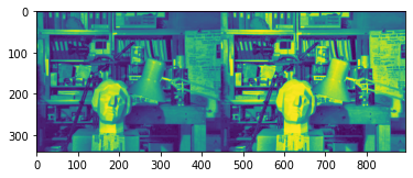
hist_full = cv2.calcHist([img], [0], None, [256], [0, 256])
hist_mask = cv2.calcHist([img], [0], mask, [256], [0, 256])
plt.subplot(221), plt.imshow(img, 'gray')
plt.subplot(222), plt.imshow(mask, 'gray')
plt.subplot(223), plt.imshow(masked_img, 'gray')
plt.subplot(224), plt.plot(hist_full), plt.plot(hist_mask)
plt.xlim([0, 256])
plt.show()

égalisation des histogrammes


img = cv2.imread('clahe.jpg',0) #0Représente un diagramme à l'échelle grise #clahe
plt.hist(img.ravel(),256);
plt.show()

equ = cv2.equalizeHist(img)
plt.hist(equ.ravel(),256)
plt.show()

res = np.hstack((img,equ))
cv_show1(res,'res')
égalisation adaptative des histogrammes
clahe = cv2.createCLAHE(clipLimit=2.0, tileGridSize=(8,8))
res_clahe = clahe.apply(img)
res = np.hstack((img,equ,res_clahe))
cv_show1(res,'res')

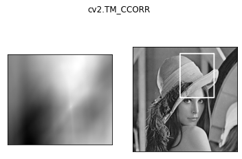
Correspondance des modèles
L'appariement des modèles et le principe de convolution sont très similaires,Le modèle glisse à partir de l'origine sur l'image originale,Modèles de calcul et(Où l'image est couverte par le modèle)Le degré de différence,Cette différence est calculée enopencv- Oui.6Espèce,Ensuite, mettez les résultats de chaque calcul dans une matrice,Comme résultat.Si le dessin original estAxBTaille,Et le modèle estaxbTaille,La matrice du résultat de sortie est(A-a+1)x(B-b+1)
# Correspondance des modèles
img = cv2.imread('lena.jpg', 0)
template = cv2.imread('face.jpg', 0)
h, w = template.shape[:2]
img.shape
(263, 263)
template.shape
(110, 85)
- TM_SQDIFF:Calculer le carré est différent,Plus la valeur calculée est faible,Plus pertinent
- TM_CCORR:Calculer la corrélation,Plus la valeur calculée est élevée,Plus pertinent
- TM_CCOEFF:Calculer le coefficient de corrélation,Plus la valeur calculée est élevée,Plus pertinent
- TM_SQDIFF_NORMED:Calculer la différence de carré normalisé,Plus la valeur calculée est proche0,Plus pertinent
- TM_CCORR_NORMED:Calculer la corrélation normalisée,Plus la valeur calculée est proche1,Plus pertinent
- TM_CCOEFF_NORMED:Calcul du coefficient de corrélation normalisé,Plus la valeur calculée est proche1,Plus pertinent
Formule:https://docs.opencv.org/3.3.1/df/dfb/group__imgproc__object.html#ga3a7850640f1fe1f58fe91a2d7583695d
methods = ['cv2.TM_CCOEFF', 'cv2.TM_CCOEFF_NORMED', 'cv2.TM_CCORR',
           'cv2.TM_CCORR_NORMED', 'cv2.TM_SQDIFF', 'cv2.TM_SQDIFF_NORMED']
res = cv2.matchTemplate(img, template, cv2.TM_SQDIFF)
res.shape
(154, 179)
min_val, max_val, min_loc, max_loc = cv2.minMaxLoc(res) #Plus la valeur est petite, mieux c'est.
min_val
39168.0
max_val
74403584.0
min_loc
(107, 89)
max_loc
(159, 62)
for meth in methods:
    img2 = img.copy()

    # La vraie valeur de la méthode de correspondance
    method = eval(meth)
    print (method)
    res = cv2.matchTemplate(img, template, method)
    min_val, max_val, min_loc, max_loc = cv2.minMaxLoc(res)

    # Si la différence carrée correspondTM_SQDIFFOu la différence carrée normalisée correspondTM_SQDIFF_NORMED,Prenez le minimum
    if method in [cv2.TM_SQDIFF, cv2.TM_SQDIFF_NORMED]:
        top_left = min_loc
    else:
        top_left = max_loc
    bottom_right = (top_left[0] + w, top_left[1] + h)

    # Dessiner un rectangle
    cv2.rectangle(img2, top_left, bottom_right, 255, 2)

    plt.subplot(121), plt.imshow(res, cmap='gray')
    plt.xticks([]), plt.yticks([])  # Cacher les axes
    plt.subplot(122), plt.imshow(img2, cmap='gray')
    plt.xticks([]), plt.yticks([])
    plt.suptitle(meth)
    plt.show()
4

5

2
3

0

1

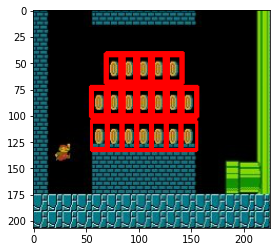
Correspond à plus d'un objet
img_rgb = cv2.imread('mario.jpg')
img_gray = cv2.cvtColor(img_rgb, cv2.COLOR_BGR2GRAY)
template = cv2.imread('mario_coin.jpg', 0)
h, w = template.shape[:2]

res = cv2.matchTemplate(img_gray, template, cv2.TM_CCOEFF_NORMED)
threshold = 0.8
# Le degré de correspondance est supérieur à%80Coordonnées de
loc = np.where(res >= threshold)
for pt in zip(*loc[::-1]):  # *Le numéro indique un paramètre optionnel
    bottom_right = (pt[0] + w, pt[1] + h)
    cv2.rectangle(img_rgb, pt, bottom_right, (0, 0, 255), 2)

cv_show(img_rgb,'img_rgb')
边栏推荐
- Embedded Software Engineer (6-15k) written examination interview experience sharing (fresh graduates)
- Idea update
- 监听iPad键盘显示和隐藏事件
- Color code
- Assembly led on
- Esp8266wifi module tutorial: punctual atom atk-esp8266 for network communication, single chip microcomputer and computer, single chip microcomputer and mobile phone to send data
- Example of offset voltage of operational amplifier
- Method of measuring ripple of switching power supply
- h5 localStorage
- "System error 5 occurred when win10 started mysql. Access denied"
猜你喜欢
![[postgraduate entrance examination] group planning: interrupted](/img/ec/1f3dc0ac22e3a80d721303864d2337.jpg)
[postgraduate entrance examination] group planning: interrupted
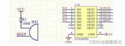
(2) Buzzer
![[postgraduate entrance examination: planning group] clarify the relationship among memory, main memory, CPU, etc](/img/c2/d1432ab6021ee9da310103cc42beb3.jpg)
[postgraduate entrance examination: planning group] clarify the relationship among memory, main memory, CPU, etc
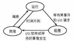
Baoyan postgraduate entrance examination interview - operating system

Go language shallow copy and deep copy

JS precompile - Variable - scope - closure

Example of offset voltage of operational amplifier
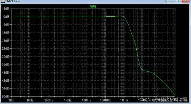
Analysis of internal circuit of operational amplifier

Cause analysis of serial communication overshoot and method of termination
X-VLM多模态模型解读
随机推荐
X-VLM多模态模型解读
(3) Dynamic digital tube
STM32 project design: temperature, humidity and air quality alarm, sharing source code and PCB
Comparison version number [leetcode]
Swift code implements method calls
Microcontroller from entry to advanced
Mapping '/var/mobile/Library/Caches/com. apple. keyboards/images/tmp. gcyBAl37' failed: 'Invalid argume
Uniapp scrolling load (one page, multiple lists)
Database learning notes I
Why are you impetuous
Relevant knowledge of DRF
leetcode2022年度刷题分类型总结(十二)并查集
"System error 5 occurred when win10 started mysql. Access denied"
Diode voltage doubling circuit
StarWar armor combined with scanning target location
static const与static constexpr的类内数据成员初始化
Pychart connects to Damon database
2022 ranking of bank financial products
[untitled]
Go language shallow copy and deep copy