Review of the paper: unmixing based soft color segmentation for image manipulation

Unmixing-Based Soft Color Segmentation for Image Manipulation Is an image processing paper based on soft segmentation , Published in SIGGRAPH 2017. The full text 19 page , In general , It's hard to understand , The article contains a lot of seemingly unrelated content , such as Matting, Iterative optimization, etc . I had a clear grasp of the article after referring to the realization of the paper .
Reference code ：https://github.com/liuguoyou/color-unmixing
B standing video：https://www.bilibili.com/video/BV1bU4y1x7MY/?vd_source=6a91312d89cec082cf6d5a92fee7279a

By convention , Take the last one teaser. For input images (a), The algorithm automatically extracts multiple layer(b), Every layer Where region Hardly intersect （ In different region The boundaries will intersect , The so-called soft segmentation ）, And each layer The color of follows a positive distribution , After extracting layers , You can adjust the color of the image , Such as (c-d) Shown .

A brief review of the classic palette based layer extraction algorithms . This kind of algorithm （Chang et al, clustering algorithm ; Tan et al, Geometric convex hull ）：
1） Firstly, several representative colors of the input image are extracted as the color palette of the image ：$C=\{C_1,C_2...C_k\}$.
2） Next, the pixels in the image are interpolated , Represent each pixel as a convex combination of palettes ：$c_p={\sum }_i{w}_i^p{C}_i$, And meet ${\sum }_i{w}_i^p=1$.
3） Each layer of nature can be represented as ：$L_i^p=w_i^p{C}_i$, among ,$L_i^p$ Represent layers $L_i$ in $p$ The color of the point .
Recoloring： according to 2）, We only need to calculate the interpolation weight once , Then modify the palette color to achieve recolor ：$c_p^{\prime }={\sum }_i{w}_i^p{C}_i^{\prime }$.

The main disadvantage of palette based algorithm is that it is difficult to maintain the sparsity of interpolation . informally , such as 2） in , Probably $p$ Interpolation weights for all palette colors $w_1^p$ All are greater than 0, In this way , When you change the color of a palette, you may change the overall color of the image , The locality of recolor operation is not good enough . Therefore, interpolation sparsity is an important problem , Sparse interpolation can achieve good local recolor . I think today's paper has achieved good sparsity to some extent , Because most pixels are associated with only one layer, not multiple , Only in region Boundary pixels are associated to multiple layers （ Be similar to matting The effect of the algorithm ）.

Back to the point , Let's briefly talk about the algorithm of this paper .

One 、 Color means

The algorithm will extract multiple layers , The color of each layer conforms to the positive distribution . Similar to palette based layer decomposition algorithm , Any layer $L_i$ contain Color and Opacity information . Pixels in the layer $p$ The color and opacity of are expressed as ：$u_i^p$ and ${\alpha }_i^p$. therefore , The color of any pixel in the image can be mixed by multiple layers ：
$$c^p=\sum _i{\alpha }_i^p{u}_i^p\text{\hspace{1em}(1)}$$
Conditions to be met 1： Guaranteed convex combination , The sum of the weights is 1： $$\sum _i{\alpha }_i^p=1\text{\hspace{1em}(2)}$$.
Conditions to be met 2： The value range of color and opacity is located in 0,1 Between ：$${\alpha }_i^p,u_i^p\in [0,1]\text{\hspace{1em}(3)}$$.

Next up , First, it introduces how to get the layer and its parameters .

Two 、 Layer decomposition

As mentioned earlier, each of the layer The color of follows a positive distribution . therefore , First of all, make sure there are several layer And estimate each layer Is a normal distribution . For the initial layer It is estimated that , This paper adopts an iterative method to automatically decide by voting layer And further estimate layer Parameters of .

1） First, put the input image in RGB The space is divided into $10\times 10\times 10=1000$ individual bins.
2） Then calculate the gradient of the image , Can be called directly Opencv Library function cv2.Laplacian Get the gradient of all pixels .
3） Traverse all pixels , For each pixel $p$, Navigate to the bin Suppose its coordinates are $b=\{b_r,b_g,b_b\}$, Calculate the voting weight of the pixel ：
$$v^p=e^{-\Vert \nabla c^p\Vert }\left(1-e^{-r^p}\right)\text{\hspace{1em}(4)}$$
among ,$\nabla c^p$ Express $p$ Gradient of ,$r^p$ It is called in the paper representation score, Think of it as $p$ The reconstruction error of , How to calculate the reconstruction error will be described later in the second part . It can be seen from the formula that ：
a) Reconstruction error $r^p$ The bigger it is ,$e^{-r^p}$ The closer the 0, thus $\left(1-e^{-r^p}\right)$ The bigger it is , Lead to $v^p$ The bigger it is .
b) gradient $\nabla c^p$ The smaller is the difference between the color of the point and the surrounding color ,$e^{-\Vert \nabla c^p\Vert }$ The bigger it is .

Next , Accumulate the voting weight of the point to the bin： $bins[b_r][b_g][b_b]+=v^p$.

4） Choose the one with the greatest voting weight bin： $bi{n}_{max}=max(bin[0][0][0],bin[0][0][[1],...bin[9][9][9])$
5） stay $bi{n}_{max}$ Select the seed point . Traverse $bi{n}_{max}$ All pixels in , For any pixel $p$, Count it $20\times 20$ How many pixels in the neighborhood of also fall on $bi{n}_{max}$ in , Write it down as $S^p$. Last , Calculate again $p$ Point score ：
$$scor{e}_p=S^p{e}^{-\Vert \nabla c^p\Vert }\text{\hspace{1em}(5)}$$
elect $bi{n}_{max}$ The pixel with the highest score is used as the seed point ：
$$s_i=\underset{p\in \text{ bin }}{\mathrm{argmax}}{\mathcal{S}}^{p}scor{e}_p\text{\hspace{1em}(6)}$$
6） Point to the seed $s_i$ Where $20\times 20$ The neighborhood performs operations similar to Gaussian filtering , Calculate the filter weight of each pixel in the neighborhood , And let the power return to one .
7） Point to the seed $s_i$ Where $20\times 20$ Neighborhood , Estimate the parameters of the positive distribution ： Mean and covariance matrices . So we got the first one layer Corresponding normal distribution .
8） repeat 1）~ 7）, Cycle stop condition ： If the vast majority （99.5%） The reconstruction error of pixels has been very small ：$r^p<{\tau }^2$, （$\tau =5$）, Then the algorithm stops .

The process diagram of iteratively selecting seed points in the previous paper , The person in the picture is the author of the paper ！

3、 ... and 、Representation Score

Input ：$n$ individual layer The corresponding positive distribution .
Output ： Calculate the of each pixel representation score.
For each pixel $p$, Its representation score By minimizing the following energy function ：
$${\mathcal{F}}_{\mathcal{S}}=\sum _i{\alpha }_i^p{\mathcal{D}}_i\left(u_i^p\right)+\sigma \left(\frac{{\sum }_i{\alpha }_i^p}{{\sum }_i({\alpha }_i^p{)}^2}-1\right)\text{\hspace{1em}(7)}$$

The energy function consists of two terms ：
1） The first one is ：${\sum }_i{\alpha }_i^p{\mathcal{D}}_i\left(u_i^p\right)$, among $D_i$ Represent layers $L_i$ The corresponding positive distribution ,${\mathcal{D}}_i\left(u_i^p\right)$ Indicates the desired color $u_i^p$ To The distribution of the Mahalanobis distance（ Markov distance ）, ${\alpha }_i^p$ Represents the desired opacity . The main purpose of this item is to find the layer in $p$ As far as possible, the color of the point follows the estimated positive distribution , Multiply by a factor ${\alpha }_i^p$ Is to weight these distances ,${\alpha }_i^p$ The larger those layers are more important , Try to obey the positive distribution of these layers , because $p$ The color of the point , Mainly determined by these layers with large opacity .

2） The second item ：$\sigma \left(\frac{{\sum }_i{\alpha }_i^p}{{\sum }_i({\alpha }_i^p{)}^2}-1\right)$ Is a sparsity constraint ,$\sigma$ It's a coefficient , Generally set as 10. From this equation we can see that , When $p$ Point opacity set about multiple layers ${\alpha }^p=\{{\alpha }_1^p,{\alpha }_2^p,{\alpha }_3^p,...{\alpha }_k^p\}$, If only one opacity is 1, The rest are all 0 when , The minimum value will be obtained 1, So that the formula （7） Of the 2 The value of the item 0. This makes the optimized opacity set sparse （ A small number of values >0）, As said at the beginning of the article , This ensures good locality of image editing .

initialization ： Investigate $p$ The color of the point in the input image , Calculate the best matching layer （ Mahalanobis distance is the smallest ）, Assuming that $L_j$, Then initialize the color and opacity respectively ：
$$u^p=\{0,0,0,...u_j^p=1,...0\},{\alpha }^p=\{0,0,0,...{\alpha }_j^p=1,...0\}\text{\hspace{1em}(8)}$$

Pay attention to energy minimization , At the same time, we need to consider the formula （1） Reconstruction error shown , The formula （2） The convex combination constraint shown , The formula （3） Value range constraints shown .

Four 、 Results comparison and summary

Finally, compare the decomposition results of the previous layer . You can see , The layer extracted in this paper has good sparsity , For example, the orange in the image （ On the left 1 Xing di 4 Column ） Very well extracted , and Tan The method of extracting oranges is located in ; Two layers （ Right side 1 Xing di 2 Column , Right side 2 Xing di 1 Column ）.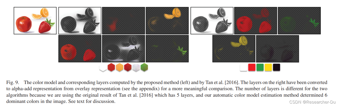

Simple summary ：
1） The method is novel , Different from the general palette decomposition algorithm , Assume that each layer follows a positive distribution ;
2） The computational complexity of the algorithm is high , It takes several iterations , It is necessary to optimize the pixel representation sore;
3） Recolor is more complex than the general palette based layer decomposition algorithm , Because this layer is not monochrome , Need to export to PS Further recolor , More trouble .
4） Personally think that , The paper is not well written , It's hard to read , Hard to understand .