当前位置:网站首页>Numpy learning notes
Numpy learning notes
2022-06-10 16:56:00 【Long way to go 2021】
NumPy(Numerical Python) It is the basic library of Scientific Computing , Provide a large number of scientific computing related functions , For example, data statistics , Random number generation, etc . The core type it provides is multidimensional array type (ndarray), Support a large number of dimension arrays and matrix operations ,Numpy Support vector processing ndarray object , Improve the operation speed of the program .
1 Basic knowledge of
Enter the command at the terminal first pip install numpy -i https://pypi.doubanio.com/simple/ download numpy, Then import to warehouse :
import numpy as np
1.1 ndarray object
NumPy Defined a n Dimensional array object , abbreviation ndarray object , It is an array set consisting of a series of elements of the same type . Each element in the array occupies a memory block of the same size .
ndarray Object adopts the index mechanism of array , Map each element in the array to a memory block , And arrange the memory blocks according to a certain layout , There are two common layout methods , That is, by row or column .
Create a ndarray Just call NumPy Of array Function :
numpy.array(object, dtype = None, copy = True, order = None, subok = False, ndmin = 0)
''' object  An array or nested sequence of numbers  dtype  Data type of array element , Optional  copy  Whether the object needs to be copied , Optional  order  Create an array style ,C In the direction of the line ,F For column direction ,A In any direction ( Default ) subok  By default, it returns an array consistent with the base class type  ndmin  Specifies the minimum dimension of the generated array  '''
1.2 data type
numpy Supported data type ratio Python There are many built-in types , Basically, it can be with C The data type of the language corresponds to , Some of the types correspond to Python Built in type . The following table lists the common NumPy Basic types .

Data type object (dtype) Is constructed using the following syntax :
numpy.dtype(object, align, copy)
- object - Data type object to convert to
- align - If true, Fill in the fields to make them look like C The structure of the body .
- copy - Copy dtype object , If false, Is a reference to a built-in data type object
An example of a structured data type is defined below student, Contains string fields name, Integer fields age, And floating point fields marks, And will the dtype Applied to the ndarray object .
import numpy as np
student = np.dtype([('name', 'S20'), ('age', 'i1'), ('marks', 'f4')])
print(student)      #  Output structured data student
ex = np.array([('abc', 21, 50), ('xyz', 18, 75)], dtype=student)    #  Apply it to ndarray object
print(ex)
Output is :
[(‘name’, ‘S20’), (‘age’, ‘i1’), (‘marks’, ‘<f4’)]
[(b’abc’, 21, 50.) (b’xyz’, 18, 75.)]
Tips : The byte order is preset by the data type < or > To decide . < It means small end method ( The minimum value is stored in the smallest address , That is, the low position group is placed in the front ).> It means big end method ( The most important bytes are stored in the smallest address , That is, the high position group is placed in the front ).
1.3 Array attribute
- size attribute : Number of array elements
array_one = np.arange(1, 100, 2)
array_two = np.random.rand(3, 4)
print(array_one.size, array_two.size)       # 50, 12
- shape attribute : The shape of the array
ndarray.shape Represents the dimensions of an array , Returns a tuple , The length of this tuple is the number of dimensions , namely ndim attribute ( Rank ). such as , A two-dimensional array , Its dimension represents " Row number " and " Number of columns ".ndarray.shape It can also be used to resize the array .
print(array_one.shape, array_two.shape) # (50,) (3, 4)
- dtype attribute : Data type of array element
print(array_one.dtype, array_two.dtype) # int32 float64
- ndim attribute : Dimension of array
print(array_one.ndim, array_two.ndim) # 1 2
- itemsize attribute : The number of bytes of memory space occupied by a single element of the array
array_three = np.arange(1, 100, 2, dtype=np.int8)
print(array_one.itemsize, array_two.itemsize, array_three.itemsize)     # 4 8 1
- nbytes attribute : The number of bytes of memory space occupied by all elements of the array
print(array_one.nbytes, array_two.nbytes, array_three.nbytes) # 200 96 50
- flat attribute : Array ( After one dimension ) Iterators for elements
from typing import Iterable
print(isinstance(array_two.flat, np.ndarray), isinstance(array_two.flat, Iterable))     # False True
- base attribute : The base object of the array ( If the array shares the memory space of other arrays )
array_four = array_one[:]
print(array_four.base is array_one, array_one.base is array_three)      # True False
Summary :
| attribute | explain |
|---|---|
| ndarray.ndim | Rank , That is, the number of axes or dimensions |
| ndarray.shape | Dimension of array , For matrices ,n That's ok m Column |
| ndarray.size | The total number of array elements , amount to .shape in n*m Value |
| ndarray.dtype | ndarray The element type of the object |
| ndarray.itemsize | ndarray The size of each element in the object , In bytes |
| ndarray.flags | ndarray Object's memory information |
| ndarray.real | ndarray The real part of the element |
| ndarray.imag | ndarray The imaginary part of the element |
| ndarray.data | Buffer containing actual array elements , Because we usually get the elements through the index of the array , So you don't usually need to use this property . |
2 Basic operation
2.1 Create array
1. One dimensional array
- Method 1 : Use
arrayfunction , adoptlistCreate an array object
array1 = np.array([1, 2, 3, 4, 5])
array1      # array([1, 2, 3, 4, 5])
- Method 2 : Use
arangefunction , Specify the value range to create an array object
array2 = np.arange(0, 20, 2)
array2      # array([ 0, 2, 4, 6, 8, 10, 12, 14, 16, 18])
- Method 3 : Use
linspacefunction , Creates an array object with evenly spaced numbers in the specified range
array3 = np.linspace(-5, 5, 101)
array3      # array([-5., -4.9, -4.8, ..., 4.8, 4.9, 5.])
- Method four : Use
numpy.randomThe function of the module generates random numbers to create array objects
produce 10 individual [ 0 , 1 ) [0, 1) [0,1) Random decimal of the range , Code :
array4 = np.random.rand(10)
array4  #
produce 10 individual [ 1 , 100 ) [1, 100) [1,100) The random integer of the range , Code :
array5 = np.random.randint(1, 100, 10)
array5      # array([29, 97, 87, 47, 39, 19, 71, 32, 79, 34])
produce 20 individual μ = 50 , σ = 10 \mu=50, \sigma=10 μ=50,σ=10 The normal distribution random number of , Code :
array6 = np.random.normal(50, 10, 20)
array6
2. Two dimensional array
- Method 1 : Use
arrayfunction , By nestinglistCreate an array object
array7 = np.array([[1, 2, 3], [4, 5, 6]])
array       # array([[1, 2, 3], [4, 5, 6]])
- Method 2 : Use
zeros、ones、full、emptyFunction to specify the shape of an array to create an array object
array8 = np.zeros((3, 4))      #  Generate 3×4 All zero array of
array9 = np.ones((3, 4))       #  Generate 3×4 All one array of
array10 = np.full((3, 4), 6)   #  Generate 3×4 Of all the 6 Array
array10 = np.empty((3, 4))     #  Generate 3×4 Uninitialized array
Tips : numpy.empty() The returned array has random values , But these values have no practical significance . Bear in mind empty Not creating an empty array .
- Method 3 : Use
eyeFunction to create an identity matrix
array11 = np.eye(4) # # Generate 4×4 The identity matrix of
- Method four : adopt
reshapeTurn a one-dimensional array into a two-dimensional array
array12 = np.array([1, 2, 3, 4, 5, 6]).reshape(2, 3)
reminder :reshape yes ndarray A method of an object , Use reshape Method to ensure that the number of array elements after shape adjustment is consistent with the number of array elements before shape adjustment , Otherwise, an exception will occur .
Add :
Sometimes array_ex.reshape(c, -1), Represents the reorganization of this matrix or array , With c That's ok d The form of column means , as follows :
arr.shape       # (a, b)
arr.reshape(m ,-1)  #  Change dimension to m That's ok 、d Column  (-1 Indicates that the number of columns is calculated automatically ,d= a*b /m )
arr.reshape(-1, m)  #  Change dimension to d That's ok 、m Column  (-1 Indicates that the number of rows is calculated automatically ,d= a*b /m )
-1 And that's what it does : Automatic calculation d:d= The number of all elements in an array or matrix /c, d It has to be an integer , Otherwise an error )
frequently-used reshape(1, -1) Convert to one line ,reshape(-1, 1) Into a column .
- Method five : adopt
numpy.randomThe function of the module generates random numbers to create array objects
array13 = np.random.rand(3, 4)      # [0,1) Range of random decimals 3 That's ok 4 Two dimensional array of columns
array14 = np.random.randint(1, 100, (3, 4))     # [1, 100) Range of random integers 3 That's ok 4 Two dimensional array of columns
3. Multidimensional arrays
- Method 1 : Create multidimensional arrays in a random way
array15 = np.random.randint(1, 100, (3, 4, 5)) # 3×4×5 Array of
- Method 2 : Shape a one-dimensional and two-dimensional array into a multi-dimensional array
array16 = np.arange(1, 25).reshape((2, 3, 4))       #  A one-dimensional array is shaped into a multi-dimensional array
array17 = np.random.randint(1, 100, (4, 6)).reshape((4, 3, 2))      #  A two-dimensional array is shaped into a multi-dimensional array
- Method 3 : Read the picture to get the corresponding three-dimensional array
from matplotlib import pyplot as plt        #  Import library
array18 = plt.imread('01.jpg')              #  Load any picture
2.2 Index and slice
NumPy Of ndarray Objects can be indexed and sliced , Through the index, you can get or modify the elements in the array , By slicing, you can extract part of the array .
- Index operation
One dimensional array
array19 = np.arange(10)
print(array19[0], array19[array19.size-1])      # 0 9
print(array19[-array19.size], array19[-1])      # 0 9
For the position of the two-dimensional array, please refer to the following figure :

array20 = np.array([[1, 2, 3], [4, 5, 6], [7, 8, 9]])
print(array20[2])       # [7 8 9]
print(array20[0][0], array20[-1][-1])       # 1 9
- Slice operation
The slice is shaped like [ Start index : End index : step ] The grammar of , Start indexing by specifying ( The default value is infinitesimal )、 End index ( The default value is infinite ) And step length ( The default value is 1), Extract the elements of the specified part from the array and form a new array . Because start indexing 、 The end index and step size have default values , So they can all be omitted , If you don't specify the step size , The second colon can also be omitted . Slice operation of one-dimensional array Python Medium list The slice of type is very similar , You can refer to the list slicing operation , The slice of a two-dimensional array can be seen in the following picture .

print(array20[:2, 1:])      # [[2 3] [5 6]]
print(array20[2])           # [7 8 9]
print(array20[2, :])        # [7 8 9]
print(array20[2:, :])       # [[7 8 9]]
print(array20[:, :2])       # [[1 2] [4 5] [7 8]]
print(array20[1, :2])       # [4 5]
print(array20[1:2, :2])     # [[4 5]]
print(array20[::2, ::2])    # [[1 3] [7 9]]
print(array20[::-2, ::-2])  # [[9 7] [3 1]]
- Fancy index
Fancy index (Fancy indexing) It refers to the use of integer arrays for indexing , The integer array mentioned here can be NumPy Of ndarray, It can also be Python in list、tuple And so on , You can use positive or negative indexes .
array22 = np.array([[30, 20, 10], [40, 60, 50], [10, 90, 80]])
array22[[0, 2]]         #  Take the second... Of the two-dimensional array 1 Xing He 3 That's ok
array22[[0, 2], [1, 2]] #  Take the second... Of the two-dimensional array 1 Xing di 2 Column , The first 3 Xing di 3 Two elements of the column  array([20, 80])
array22[[0, 2], 1]      #  Take the second... Of the two-dimensional array 1 Xing di 2 Column , The first 3 Xing di 2 Two elements of the column  array([20, 90])

- Boolean index
Boolean index is to index array elements through Boolean array , Boolean arrays can be constructed manually , You can also generate boolean arrays through relational operations .
array23 = np.arange(1, 10)
array23[[True, False, True, True, False, False, False, False, True]]    # array([1, 3, 4, 9])
array23 >= 5    # array([False, False, False, False, True, True, True, True, True])
~(array23 >= 5) # ~ Operator can realize logical inversion ,array([ True, True, True, True, False, False, False, False, False])
array23[array23 >= 5]   # array([5, 6, 7, 8, 9])
reminder : Slicing creates a new array object , But the new array and the original array share the data in the array , To put it simply , If you modify the data in the array through the new array object or the original array object , In fact, the same piece of data is modified . Fancy and Boolean indexes also create new array objects , And the new array duplicates the elements of the original array , The new array and the original array do not share data , This is achieved through the array base Properties also let you know , Pay attention when using .
2.3 Broadcast mechanism
radio broadcast (Broadcast) yes numpy For different shapes (shape) How to do the numerical calculation of the array , Arithmetic operations on arrays are usually performed on the corresponding elements .
If two arrays array23 and array25 The same shape , The meet array24.shape == array25.shape, that array24*array25 The result is that array24 And array25 Array corresponding bit multiplication . This requires the same dimension , And the length of each dimension is the same .
array24 = np.array([1, 2, 3, 4])
array25 = np.array([10, 20, 30, 40])
array26 = array24 * array25
print(array26)        # [10 40 90 160]
When in operation 2 The shapes of arrays are different ,numpy Will automatically trigger the broadcast mechanism . Such as :
array27 = np.array([[ 0, 0, 0],
           [10,10,10],
           [20,20,20],
           [30,30,30]])
array28 = np.array([1,2,3])
print(array27 + array28)
The result is shown in the figure below :


2.4 Traversal array
NumPy Iterator object numpy.nditer Provides a flexible way to access one or more array elements , Can cooperate with for Loop completes the traversal of array elements . Example 1 :
array29 = np.arange(0,60,5)
array29 = array29.reshape(3,4)
for x in np.nditer(array26):      #  Use nditer iterator , And use for Traversal
   print(x)     # 0 5 10 15 20 25 30 35 40 45 50 55
In memory ,Numpy Arrays provide two ways to store data , Namely C-order( Row precedence ) And Fortrant-order( List priorities ).nditer The iterator chooses an order consistent with the array memory layout , The reason for doing this , To improve data access efficiency .
By default , When we traverse the elements in the array , There is no need to consider the storage order of the array , This can be verified by traversing the transposed array of the above array . Example 2 :
array30 = np.arange(0,60,5)
array30 = array30.reshape(3,4)
array31 = array30.T     # a Transpose array
for x in np.nditer(array31):
   print(x,end=",")        # a Transposed traversal output  0 5 10 15 20 25 30 35 40 45 50 55
Let's say C Style to access a copy of the transposed array . Example 3 as follows :
array32 = np.arange(0,60,5).reshape(3,4)
for x in np.nditer(array32.T.copy(order='C')):        # copy Method to generate a copy of the array
    print (x, end=", " )        # 0, 20, 40, 5, 25, 45, 10, 30, 50, 15, 35, 55,
Control traversal order
- for x in np.nditer(array, order=‘F’):Fortran order, That is, sequence first ;
- for x in np.nditer(array30.T, order=‘C’):C order, That is, line order takes precedence ;
array33 = np.arange(0,60,5)
array33 = array33.reshape(3,4)
print(array33)
for x in np.nditer(array33, order = 'C'):
   print (x,end=",")    # C-order Line order  0,5,10,15,20,25,30,35,40,45,50,55,
for x in np.nditer(array33, order = 'F'):
   print (x,end=",")    # F-order Column order  0,20,40,5,25,45,10,30,50,15,35,55,
2.5 other
| The name of the function | Function introduction |
|---|---|
reshape | Without changing the elements of the array , Modify the shape of the array . |
flat | Return is an iterator , It can be used for Loop through each of these elements . |
flatten | Returns a copy of the array in the form of a one-dimensional array , The operation on the copy will not affect the original array . |
ravel | Returns a continuous flat array ( That is, the expanded one-dimensional array ), And flatten Different , It returns an array view ( Modifying the view will affect the original array ). |
| The name of the function | Function introduction |
|---|---|
transpose | Swap the dimension values of the array , For example, two-dimensional array dimension (2,4) After using this method, it is (4,2) |
ndarray.T | And transpose In the same way |
rollaxis | Roll back to the specified position along the specified axis |
swapaxes | Swap the axes of the array |
| The name of the function | Function introduction |
|---|---|
resize | Returns a new array of specified shapes |
append | Add values to the end of the array |
insert | Inserts the element value in front of the specified element along the specified axis |
delete | Delete the subarray of a certain axis , And return the new array after deletion |
unique | Used to delete duplicate elements in the array , And return a new array according to the element value from large to small |
notes :resize Only modify the original array , no return value , and reshape Not only modify the original array , At the same time, the modified results are returned .
Numpy Array operation : Modify array shape 、 Flip array 、 Modify array dimensions 、 Linked array 、 Split array 、 Addition and deletion of array elements , Read more :https://www.runoob.com/numpy/numpy-array-manipulation.html
3 Common functions
3.1 General univariate function
The general function is right ndarray A function that performs element-level operations on the data in . You can think of it as a normal function ( Take a scalar value as a parameter , Returns a scalar value ) Vectorized wrapper , As shown below .
| function | explain |
|---|---|
abs / fabs | A function of absolute value |
sqrt | The function of finding the square root , amount to array ** 0.5 |
square | The function of finding the square , amount to array ** 2 |
exp | Calculation e x e^x ex Function of |
log / log10 / log2 | Logarithmic function (e Bottom / 10 Bottom / 2 Bottom ) |
sign | Symbolic function (1 - Positive numbers ;0 - zero ;-1 - negative ) |
ceil / floor | Round up / Round down |
isnan | Returns a Boolean array ,NaN Corresponding True, Not NaN Corresponding False |
isfinite / isinf | Determine whether the value is a function of infinity |
cos / cosh / sin | Trigonometric functions |
sinh / tan / tanh | Trigonometric functions |
arccos / arccosh / arcsin | Anti trigonometric function |
arcsinh / arctan / arctanh | Anti trigonometric function |
rint / round | Round function |
array34 = np.array([0, 30, 45, 60, 90])
print(np.sin(array34*np.pi/180))    # [0. 0.5 0.70710678 0.8660254 1.]
3.2 General binary function
| function | explain |
|---|---|
add(x, y) / substract(x, y) | Addition function / Subtraction function |
multiply(x, y) / divide(x, y) | Multiplication function / Division function |
floor_divide(x, y) / mod(x, y) | Integral division function / Find the modular function |
allclose(x, y) | Check the array x and y Whether the elements are almost equal |
power(x, y) | Array x x x The elements of x i x_i xi And an array y y y The elements of y i y_i yi, Calculation x i y i x_i^{y_i} xiyi |
maximum(x, y) / fmax(x, y) | Compare elements in pairs to get the maximum value / Get the maximum ( Ignore NaN) |
minimum(x, y) / fmin(x, y) | Compare elements in pairs to get the minimum value / Get the minimum ( Ignore NaN) |
inner(x, y) | Inner product operation |
cross(x, y) / outer(x, y) | Cross product operations / Outer product operation |
intersect1d(x, y) | Calculation x and y Intersection , Returns an ordered array of these elements |
union1d(x, y) | Calculation x and y Union , Returns an ordered array of these elements |
in1d(x, y) | Return to the judgment of x Whether the element of is in y An array of Boolean values obtained in |
setdiff1d(x, y) | Calculation x and y The difference between the set , Returns an array of these elements |
setxor1d(x, y) | Calculation x and y Symmetry difference of , Returns an array of these elements |
Additional explanation : In two dimensions , Two vectors A = [ a 1 a 2 ] \boldsymbol{A}=\begin{bmatrix} a_1 \\ a_2 \end{bmatrix} A=[a1a2] and B = [ b 1 b 2 ] \boldsymbol{B}=\begin{bmatrix} b_1 \\ b_2 \end{bmatrix} B=[b1b2] The cross product of is defined like this : A × B = ∣ a 1 a 2 b 1 b 2 ∣ = a 1 b 2 − a 2 b 1 \boldsymbol{A}\times \boldsymbol{B}=\begin{vmatrix} a_1 \quad a_2 \\ b_1 \quad b_2 \end{vmatrix}=a_1b_2 - a_2b_1 A×B=∣∣∣∣a1a2b1b2∣∣∣∣=a1b2−a2b1, among ∣ a 1 a 2 b 1 b 2 ∣ \begin{vmatrix} a_1 \quad a_2 \\ b_1 \quad b_2 \end{vmatrix} ∣∣∣∣a1a2b1b2∣∣∣∣ It's called a determinant . But be sure to pay attention to , Cross product is not equivalent to determinant , The result of a determinant is a scalar , The result of the cross product operation is a vector . If you don't understand , We can look at two vectors in three-dimensional space , A = [ a 1 a 2 a 3 ] \boldsymbol{A}=\begin{bmatrix} a_1 \\ a_2 \\ a_3 \end{bmatrix} A=⎣⎡a1a2a3⎦⎤ and B = [ b 1 b 2 b 3 ] \boldsymbol{B}=\begin{bmatrix} b_1 \\ b_2 \\ b_3 \end{bmatrix} B=⎣⎡b1b2b3⎦⎤ The cross product of is < i ^ ∣ a 2 a 3 b 2 b 3 ∣ , − j ^ ∣ a 1 a 3 b 1 b 3 ∣ , k ^ ∣ a 1 a 2 b 1 b 2 ∣ > \left< \hat{i} \begin{vmatrix} a_2 \quad a_3 \\ b_2 \quad b_3 \end{vmatrix}, -\hat{j} \begin{vmatrix} a_1 \quad a_3 \\ b_1 \quad b_3 \end{vmatrix}, \hat{k} \begin{vmatrix} a_1 \quad a_2 \\ b_1 \quad b_2 \end{vmatrix} \right> *i^∣∣∣∣a2a3b2b3∣∣∣∣,−j^∣∣∣∣a1a3b1b3∣∣∣∣,k^∣∣∣∣a1a2b1b2∣∣∣∣*, among i ^ , j ^ , k ^ \hat{i}, \hat{j}, \hat{k} i^,j^,k^ The unit vector representing each dimension .
array36 = np.array([10, 20, 30])
array37 = np.array([3, 5, 7])
print(np.mod(array36, array37))  # [1 0 2]
3.3 Statistical function
Statistical methods mainly include :sum()、mean()、std()、var()、min()、max()、argmin()、argmax()、cumsum() etc. , Respectively used to sum the elements in the array 、 Averaging 、 Find standard deviation 、 Variance estimation 、 Find maximum 、 Look for the smallest 、 Find the cumulative sum, etc , Please refer to the following code .
array38 = np.array([1, 2, 3, 4, 5, 5, 4, 3, 2, 1])
print(array38.sum())        # 30
print(array38.mean())       # 3.0
print(array38.max())        # 5
print(array38.min())        # 1
print(array38.std())        # 1.4142135623730951
print(array38.var())        # 2.0
print(array38.cumsum())     # [ 1 3 6 10 15 20 24 27 29 30]
all() / any()Method : Determine whether all elements of the array are True / Determine whether the array has a as True The elements of .astype()Method : Copy an array , And convert the elements in the array to the specified type .dot()Method : Realize dot product operation of an array and another array .
4 Math library
4.1 Matrix library
NumPy For linear algebra (linear algebra) Module and type of representation matrix matrix, Of course, we can also express a matrix through a two-dimensional array , The official does not recommend the use of matrix Class, but a two-dimensional array is recommended , And it is possible that it will be removed in future versions matrix class .NumPy Contains a matrix library numpy.matlib, The function in this module returns a matrix , instead of ndarray object .
| The name of the function | Function introduction |
|---|---|
matlib.empty() | Returns an empty matrix , So its creation speed is very fast |
numpy.matlib.zeros() | Create a to 0 Filled matrix |
numpy.matlib.ones() | Create a to 1 Filled matrix |
numpy.matlib.eye() | Returns a diagonal element that is 1, The other elements are 0 Matrix |
numpy.matlib.identity() | Returns an identity matrix of a given size , The diagonal elements of the matrix are 1, Other elements are 0 |
numpy.matlib.rand() | Create one filled with random numbers , And give a matrix of dimensions |
4.2 linear algebra
NumPy Provides numpy.linalg modular , This module contains some commonly used linear algebra calculation methods
| function | explain |
|---|---|
diag | Return the diagonal elements of a square array in the form of a one-dimensional array or convert a one-dimensional array into a square array ( Off diagonal elements are 0) |
vdot | The dot product of vectors |
dot | Dot product of array |
inner | Inner product of array |
outer | The cross product of an array |
trace | Calculate the sum of the diagonal elements |
norm | modulus ( norm ) operation |
det | Calculate the value of the determinant ( If you calculate on a square matrix, you will get a scalar ) |
matrix_rank | Calculate the rank of the matrix |
eig | Calculate the eigenvalues of the matrix (eigenvalue) And eigenvectors (eigenvector) |
inv | Calculate the nonsingular matrix ( n n n Square matrix ) The inverse matrix |
pinv | Calculate the mole of the matrix - Penrose (Moore-Penrose) Generalized inverse |
qr | QR decompose ( The matrix is decomposed into the product of an orthogonal matrix and an upper triangular matrix ) |
svd | Calculate singular value decomposition (singular value decomposition) |
solve | Solve a system of linear equations A x = b \boldsymbol{A}\boldsymbol{x}=\boldsymbol{b} Ax=b, among A \boldsymbol{A} A It's a square array |
lstsq | Calculation A x = b \boldsymbol{A}\boldsymbol{x}=\boldsymbol{b} Ax=b The least square solution of |
Important concepts
1. Copies and views
A replica is a complete copy of data , If we modify the copy , It doesn't affect the raw data , Physical memory is not in the same location .
A view is a nickname or reference to data , Through this nickname or reference, you can also access 、 Manipulate the original data , But the original data will not be copied . If we modify the view , It affects the raw data , The physical memory is in the same location .
Views generally occur in :
- numpy The slicing operation returns the view of the original data .
- call ndarray Of
view()Function to generate a view .
Copies usually occur in :
- Python Sequence slicing , call
deepCopy()function . - call ndarray Of
copy()The function produces a copy .
2. Byte swapping
On almost all machines , Multibyte objects are stored as a sequence of consecutive bytes . Byte order , Is a storage rule for program objects that span multiple bytes .
- Big end model : The high byte of data is stored in the low address of memory , The low byte of data is stored in the high address of memory , This kind of storage mode is a bit similar to processing data in string order : The address increases from small to large , And the data goes from high to low ; This is consistent with our reading habits .
- The small end model : The high byte of data is stored in the high address of memory , And the low byte of data is stored in the low address of memory , This storage mode effectively combines the high and low address with the data bit weight , The weight of high address part is high , The weight of low address part is low .
Add :
NumPy Usually deal with more real numbers , For strings 、 Binary operation 、IO operation , You can refer to :NumPy String function :https://www.runoob.com/numpy/numpy-string-functions.html、NumPy An operation https://www.runoob.com/numpy/numpy-binary-operators.html、IO operation https://www.runoob.com/numpy/numpy-linear-algebra.html
Reference resources
- Python And numpy Detailed tutorial :https://blog.csdn.net/qq_46092061/article/details/118410838
- Numpy course :https://www.runoob.com/numpy/numpy-tutorial.html
- Numpy:http://c.biancheng.net/numpy/what-is-numpy.html
- The most comprehensive NumPy course :https://blog.51cto.com/python3/2950582
边栏推荐
- Build a leading privacy computing scheme impulse online data interconnection platform and obtain Kunpeng validated certification
- Simple file upload
- Why__ Inline usually needs static
- Research Report on the application field of Chinese antirust oil market and the prospect planning of the 14th five year plan (2022-2028)
- 【Proteus仿真】DS18B20+报警温度可调+LM016显示
- 线程面试相关问题
- Desai wisdom number - words (text wall): 25 kinds of popular toys for the post-80s children
- 亦舒作品经典语句
- Detailed steps for installing redis image in docker (easy to understand, suitable for novices to get started quickly)
- Only by truly finding the right way to land and practice the meta universe can we ensure the steady and long-term development
猜你喜欢
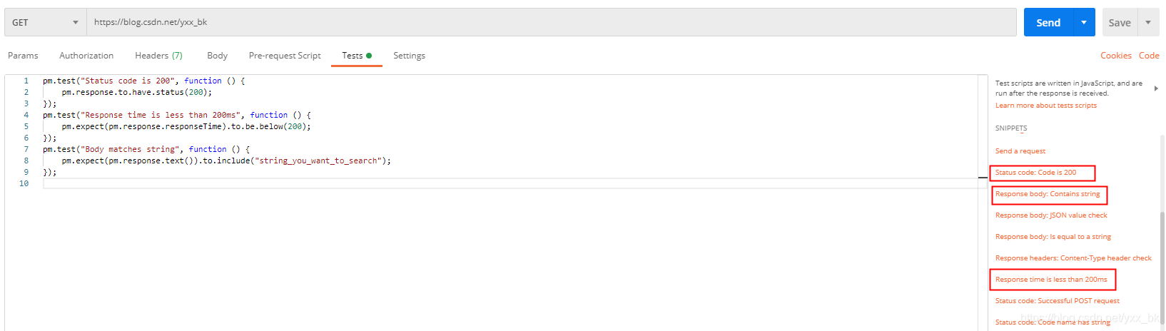
postman常用断言

Report on development status and investment planning recommendations of global and Chinese fuel filler pipe markets (2022-2028)

Fosun Group hekaiduo: grow together with Alibaba cloud and help business innovation

Enroulez - vous, brisez l'anxiété de 35 ans, l'animation montre le processeur enregistrer le processus d'appel de fonction, entrer dans l'usine d'interconnexion est si simple

嵌入式开发:使用MCU进行无线更新面临的5大挑战

解决idea打开某个项目卡住的问题

Introduction to postmangrpc function
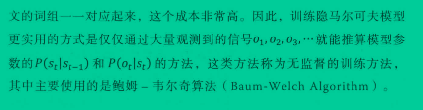
隐形马尔可夫模型及其训练(一)

提高效率的 5 个 GoLand 快捷键,你都知道吗?
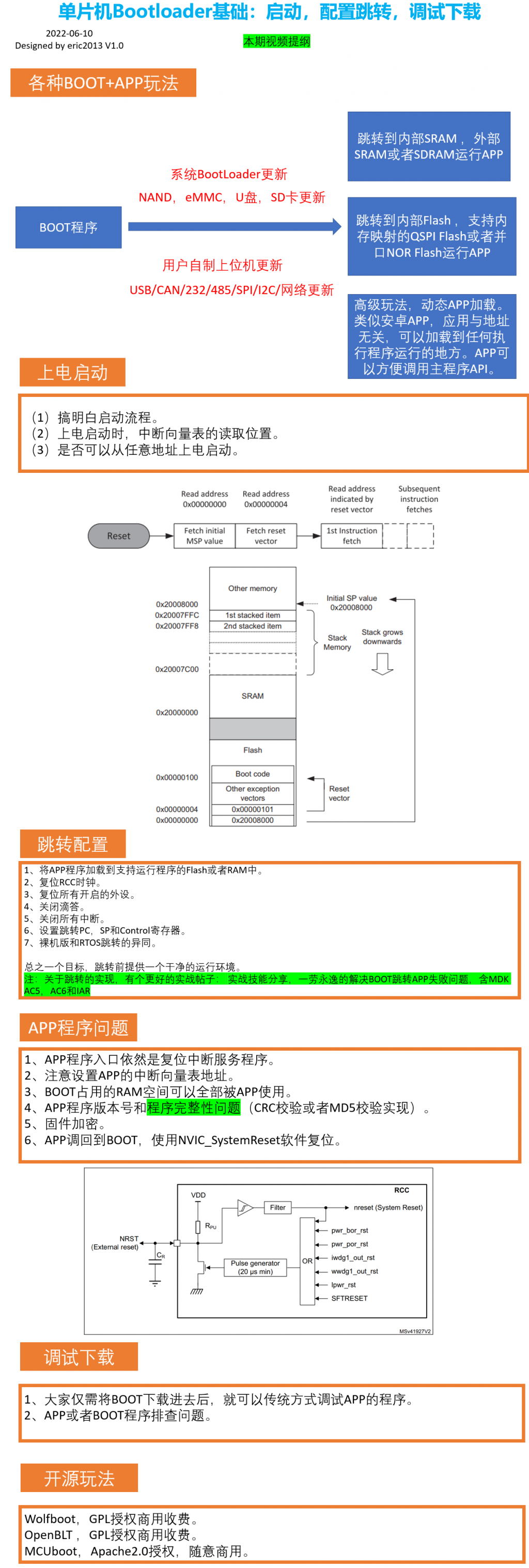
【BSP视频教程】BSP视频教程第17期:单片机bootloader专题,启动,跳转配置和调试下载的各种用法(2022-06-10)
随机推荐
Quickly understand the commonly used symmetric encryption algorithm, and no longer have to worry about the interviewer's thorough inquiry
[quick code] define the new speed of intelligent transportation with low code
简单实现文件上传
Basic use cases for jedis
Analysis report on market demand trend and sales strategy of global and Chinese automatic marshmallow machines (2022-2028)
Postman switching topics
Zhangxiaobai teaches you how to use Ogg to synchronize Oracle 19C data with MySQL 5.7 (3)
Only by truly finding the right way to land and practice the meta universe can we ensure the steady and long-term development
Effect comparison and code implementation of three time series hybrid modeling methods
PyTorch基础(一)-- Anaconda 和 PyTorch安装
AI video cloud: a good wife in the era of we media
fail-fast和fail-safe
VBA判断一个长字符串中是否包含另一个短字符串
复利最高的保险产品是什么?一年要交多少钱?
靠,嘉立创打板又降价
Technology sharing | quick intercom, global intercom
Cannot locate a 64-bit Oracle Client library:The specified module could not be found.
Web2 到 Web3,意识形态也需要发生改变
数字图像处理:灰度化
Zhangxiaobai teaches you how to use Ogg to synchronize Oracle 19C data with MySQL 5.7 (2)