NLP introduction + practice: Chapter 4: using pytorch to manually realize linear regression

Last one ： 《nlp introduction + actual combat ： The third chapter ： Gradient descent and back propagation 》

Code link of this chapter ：

• https://gitee.com/ninesuntec/nlp-entry-practice/blob/master/code/4. Use pytorch Complete linear regression .py
• https://gitee.com/ninesuntec/nlp-entry-practice/blob/master/code/4. Manual implementation of linear regression .py

1. Forward calculation

about pytorch One of them tensor, If you set its properties .requires_grad by True, Then it will track all operations for this submission . Or it can be understood as , This tensor It's a parameter , The gradient will be calculated later , Update this parameter .

1.1 The calculation process

Suppose the following conditions (1/4 Mean value ,xi There is 4 Number ), Use torch The process of completing its forward calculation .
$$\begin{gathered} o=\frac{1}{4}\sum _i{z}_i \\ {z}_i=3(x_i+2{)}^2 \end{gathered}$$
among ：
$$Z_i(x_i=1)=27$$
If x Is the parameter , The gradient needs to be calculated and updated

that , Set randomly at the beginning x The value of , Need to set his requires_grad The attribute is True, The default value is None

import torch

x = torch.ones(2, 2, requires_grad=True)  #  Initialize parameters x, And set up requires_grad=True Used to track its calculation history 
print("x=", x)
y = x + 2
print("y=", y)
z = y * y * 3  #  square *3
print("z=", z)
out = z.mean()  #  Calculating mean 
print("out=", out)

As can be seen from the above code :

• 1.x Of requires_grad The attribute is True
• 2. Each subsequent calculation will modify its grad_fn attribute , Used to record operations done
  • 1. Through this function and grad_fn It can form a calculation diagram similar to that in the previous chapter

1.2 requires_grade and grad_fn

a = torch.randn(2, 2)
a = ((a * 3) / (a - 1))
print(a.requires_grad)
a.requires_grad_(True)  #  Modify in place 
print(a.requires_grad)
b = (a * a).sum()
print(b.requires_grad)
with torch.no_grad():
    c = (a * a).sum()
print(c.requires_grad)

Be careful ：

To prevent tracking history ( And using memory ), You can wrap code blocks in with torch.no_grad(): in . Especially useful when evaluating models , Because the model may have requires_grad = True Trainable parameters , But we don't need to calculate the gradient of them in the process .

2. Gradient calculation

about 1.1 Medium out for , We can use backward Method for back propagation , Calculate the gradient out.backward(), Then we can find the derivative $\frac{d_{out}}{d_x}$, call x.gard Can get the derivative value

out.backward()  #  Back propagation 
print(" Back propagation ：", x.grad)  # x.grad Get the gradient 

because ：
$$\frac{d(O)}{d(x_i)}=\frac{1}{4}\ast 6(x_i+2)=\frac{3}{2}(x_i+2)$$
stay $x_i=1$ when , Its value is 4.5

Be careful : When the output is a scalar , We can call the output tensor Of backword() Method , But when the data is a vector , call backward() You also need to pass in other parameters .

Many times our loss function is a scalar , So we won't introduce the case where the loss is a vector .

loss.backward() Is based on the loss function , For parameters (requires_grad=True) To calculate his gradient , And put it Cumulative save To x.gard , Its gradient has not been updated at this time , So you need to set the gradient to 0 After that, a new back propagation is carried out .

Be careful ：

• 1.tensor.data:
  • stay tensor Of require grad=False,tensor.data and tensor Equivalent
  • require_grad=True when ,tensor.data Just to get tensor Data in

print(a)
print(a.data)

• 2.tensor.numpy():
  • require_grad=True Cannot convert directly , Need to use tensor.detach().numpy(), let me put it another way ,tensor.detach().numpy() Be able to achieve the right tensor Deep copy of data , Turn into ndarray

3. Manually complete the implementation of linear regression

below , We use a custom data , To use torch Implement a simple linear regression
Suppose our basic model is y = wx+b
among w and b All parameters , We use y = 3x+0.8 To construct data x、y, So finally, through the model, we should be able to get w and b Should be close to 3 and 0.8

• 1. Prepare the data
• 2. Calculate the predicted value
• 3. Calculate the loss , Set the gradient of the parameter to 0, Back propagation
• 4. Update parameters

Before completing this section , We need to install a graphical display package ：matplotlib
I can go through pip install matplotlib Installation , I was directly in anaconda Installed in , Everyone according to their own needs , No, you can baidu by yourself

import torch
import numpy as np
from matplotlib import pyplot as plt

learning_rate = 0.01
# 1. Prepare the data  y=3x+0.8, Prepare parameters 
x = torch.rand([500, 1])  # 1 rank ,50 That's ok 1 Column 
y = 3 * x + 0.8
# 2. By model calculation y_predict
w = torch.rand([1, 1], requires_grad=True)
b = torch.tensor(0, requires_grad=True, dtype=torch.float32)
y_predict = x * w + b

# 4. Through the loop , Back propagation , Update parameters 
for i in range(50):  #  Training 3000 Time 
    #  Calculate the predicted value 
    y_predict = x * w + b
    # 3. Calculation loss
    loss = (y_predict - y).pow(2).mean()
    if w.grad is not None:
        w.grad.data.zero_()
    if b.grad is not None:
        b.grad.data.zero_()
    loss.backward()  #  Back propagation 
    w.data = w.data - learning_rate * w.grad
    b.data = b.data - learning_rate * b.grad
    print("w:{},b:{},loss:{}".format(w.item(), b.item(), loss.item()))
plt.figure(figsize=(20, 8))
plt.scatter(x.numpy().reshape(-1), y.numpy().reshape(-1))  #  Scatter plot 
y_predict = x * w + b
# y_predict contain gard, So we need to make a deep copy and then transfer numpy
plt.plot(x.numpy().reshape(-1), y_predict.detach().numpy().reshape(-1),color = "red",linewidth=2,label="predict")  #  A straight line 
plt.show()

Let me explain ：numpy().reshape(-1)
z.reshape(-1) or z.reshape(1,-1) Tile the array horizontally

z.reshape(-1)
array([ 1,  2,  3,  4,  5,  6,  7,  8,  9, 10, 11, 12, 13, 14, 15, 16])

z.reshape(-1, 1) Tile the array vertically

z.reshape(-1,1)
 array([[ 1],
        [ 2],
        [ 3],
        [ 4],
        [ 5],
        [ 6],
        [ 7],
        [ 8],
        [ 9],
        [10],
        [11],
        [12],
        [13],
        [14],
        [15],
        [16]])

Let's set the training times to 50 Time , After running, you can see the deviation between the predicted value and the real value ：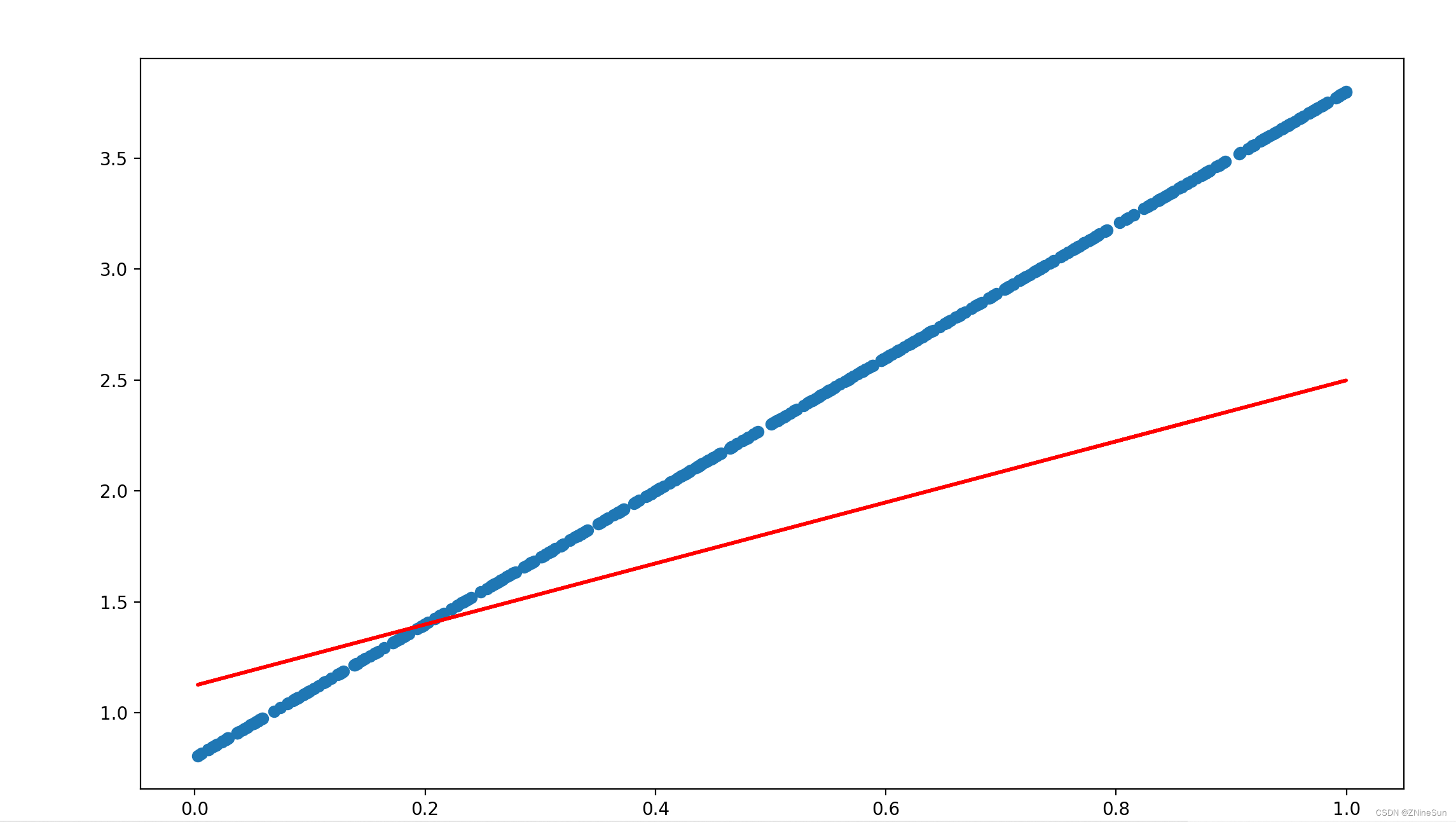

Adjust the training times to 5000 Time , You can see ：

It can be seen that the predicted result is basically close to the real value