当前位置:网站首页>[signals and systems] (XXI) Laplace transform and complex frequency domain analysis -- Laplace transform and its properties
[signals and systems] (XXI) Laplace transform and complex frequency domain analysis -- Laplace transform and its properties
2022-06-11 23:39:00 【Binary artificial intelligence】
List of articles
- Laplace transform and its properties
- 1 Definition of bilateral Laplace transform
- 2 Convergence domain
- 3 ( Causal signals ) Definition of unilateral Laplace transform
- 4 The relationship between unilateral Laplace transform and Fourier transform
- 5 Laplace transform of common signals
- 6 Properties of Laplace transform
- 7 Inverse Laplace transform
Laplace transform and its properties
The Fourier transform : j w jw jw
Laplace transform : s = σ + j w s=\sigma+jw s=σ+jw
1 Definition of bilateral Laplace transform
Some functions do not satisfy the absolute integrability condition , It is difficult to solve Fourier transform . So , An attenuation factor can be used e − σ t e^{-\sigma t} e−σt( σ \sigma σ Is a real constant ) Multiply signal f ( t ) f(t) f(t), Choose... Appropriately σ \sigma σ Value , Make the product signal f ( t ) e − σ t f(t)e^{-\sigma t} f(t)e−σt When t → ∞ t\rightarrow \infty t→∞ The signal amplitude approaches 0 , So that f ( t ) e − σ t f(t)e^{-\sigma t} f(t)e−σt The Fourier transform of exists .

The corresponding inverse Fourier transform is :


2 Convergence domain
Only choose the right σ \sigma σ Value to make the integral converge , The signal f ( t ) f(t) f(t) The bilateral Laplace transform of exists .
Convergence domain : send f ( t ) f(t) f(t) The existence of Laplace transform σ \sigma σ Value range .
2.1 Causal signals

The convergence domain of causal signal is to the right of a straight line .
2.2 Anti causal signals

The convergence domain of anti causal signal is to the left of a certain straight line .
2.3 Bilateral signals

The convergence region of bilateral signal is between two straight lines .
Conclusion :
(1) For the bilateral Laplace transform , F b ( s ) F_b(s) Fb(s) Together with the convergence domain , It can be uniquely determined that f ( t ) f(t) f(t). namely :

(2) Different signals can have the same F b ( s ) F_b(s) Fb(s), But the convergence domain is different .
3 ( Causal signals ) Definition of unilateral Laplace transform
The signals we usually encounter have initial moments , Let's set its initial time as the coordinate origin . such , t < 0 t<0 t<0 when , f ( t ) = 0 f(t)=0 f(t)=0. So the Laplace transformation is written as
F ( s ) = ∫ 0 − ∞ f ( t ) e − s t d t F(s)=\int_{0_{-}}^{\infty} f(t) \mathrm{e}^{-s t} \mathrm{~d} t F(s)=∫0−∞f(t)e−st dt
It is called unilateral Laplace transform . Laplace transform for short . Its convergence region must be R e [ s ] > α Re[s]>\alpha Re[s]>α, It can be omitted .

ε ( t ) \varepsilon(t) ε(t): unilateral , t t t Less than zero f ( t ) f(t) f(t) Value is zero .
4 The relationship between unilateral Laplace transform and Fourier transform


remarks :
∫ 1 a 2 + x 2 d x = 1 a arctan x a + C \int \frac{1}{a^{2}+x^{2}} d x=\frac{1}{a} \arctan \frac{x}{a}+C ∫a2+x21dx=a1arctanax+C
When w ≠ 0 w\not = 0 w=0 when ,
lim σ → 0 σ σ 2 + ω 2 = 0 = π δ ( ω ) \lim _{\sigma \rightarrow 0} \frac{\sigma}{\sigma^{2}+\omega^{2}}=0=\pi\delta(\omega) σ→0limσ2+ω2σ=0=πδ(ω)
When w = 0 w= 0 w=0 when , The limit value is infinity , Equivalent to impulse function δ ( w ) \delta(w) δ(w), Area is π \pi π:
∫ − ∞ ∞ σ σ 2 + ω 2 d ω = arctan ( x σ ) ∣ − ∞ + ∞ = π \int_{-\infty}^{\infty}\frac{\sigma}{\sigma^{2}+\omega^{2}}d\omega= \arctan (\frac{x}{\sigma})|_{-\infty}^{+\infty}=\pi ∫−∞∞σ2+ω2σdω=arctan(σx)∣−∞+∞=π
namely π δ ( w ) \pi\delta(w) πδ(w).

5 Laplace transform of common signals


6 Properties of Laplace transform
6.1 linear 、 Scale transformation


6.2 Time shift 、 Complex frequency shift characteristics


6.3 Calculus characteristics in time domain and complex frequency domain


We can find the Laplace transform of the original function by finding the Laplace transform of the reciprocal of the original function .


6.4 Convolution theorem

6.5 initial value 、 The final value theorem


7 Inverse Laplace transform
Directly use the definition to find the inverse transformation — Integral of complex variable function , More difficult . Common methods :
(1) Look up the table ;
(2) Utilization property ;
(3) Partial fraction expansion ----- combination
Image function F ( s ) F(s) F(s) yes s s s Rational fraction of , Can be written as 
if m ≥ n m ≥ n m≥n ( False fraction ), The image function can be divided by polynomial F ( s ) F(s) F(s) Decompose into rational polynomials P ( s ) + Yes The reason is really branch type P(s)+ Rational proper fraction P(s)+ Yes The reason is really branch type

for example :
P ( s ) P(s) P(s) The inverse Laplace transform consists of the impulse function ( δ \delta δ) And its derivatives ( δ ′ \delta' δ′, δ ′ ′ \delta'' δ′′…) constitute .
The following mainly discusses the rational proper fraction .
Partial fraction expansion 


1 s − ( − α + j β ) → e ( − α + j β ) t \frac{1}{s-(-\alpha+j\beta)}\rightarrow e^{(-\alpha+j\beta)t} s−(−α+jβ)1→e(−α+jβ)t
1 s − ( − α − j β ) → e ( − α − j β ) t \frac{1}{s-(-\alpha-j\beta)}\rightarrow e^{(-\alpha-j\beta)t} s−(−α−jβ)1→e(−α−jβ)t
By Euler formula , obtain :
e j θ ⋅ e ( − α + j β ) t + e − j θ ⋅ e ( − α − j β ) t e^{j\theta}\cdot e^{(-\alpha+j\beta)t}+e^{-j\theta}\cdot e^{(-\alpha-j\beta)t} ejθ⋅e(−α+jβ)t+e−jθ⋅e(−α−jβ)t
= e − α ( e j ( θ + β t ) + e − j ( θ + β t ) ) =e^{-\alpha}(e^{j(\theta+\beta t)}+e^{-j(\theta+\beta t)}) =e−α(ej(θ+βt)+e−j(θ+βt))
= 2 e − α cos ( β t + θ ) =2e^{-\alpha}\cos(\beta t+\theta) =2e−αcos(βt+θ)
True fraction :

False fraction :


University of China MOOC: Signals and systems , Xi'an University of Electronic Science and Technology , Bao Long Guo , Zhu JUANJUAN
边栏推荐
- Introduction and installation steps of sonarqube
- 【自然语言处理】【多模态】ALBEF:基于动量蒸馏的视觉语言表示学习
- MySQL 8.0 解压版安装教程
- Solr之基礎講解入門
- Node version control tool NVM
- sonarqube介绍和安装步骤
- Lake shore vnf series low temperature thermostat system - sample in flowing steam
- 2022年低压电工上岗证题目及在线模拟考试
- Antigen products enter the family, and Chinese medical device enterprises usher in a new blue ocean
- 2022年安全員-A證考題模擬考試平臺操作
猜你喜欢
CVPR 2022 | meta learning performance in image regression task
CVPR 2022 | 元学习在图像回归任务的表现

MySQL 8.0 decompressed version installation tutorial

产品力进阶新作,全新第三代荣威RX5盲订开启

Lake Shore—SuperTran-VP 连续流低温恒温器系统
![[day15 literature extensive reading] numerical magnetic effects temporary memories but not time encoding](/img/57/9ce851636b927813a55faedb4ecd48.png)
[day15 literature extensive reading] numerical magnetic effects temporary memories but not time encoding

2022年起重机司机(限桥式起重机)考试题模拟考试题库及模拟考试

CD流程
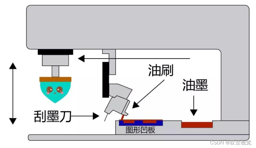
移印工艺流程及应用注意事项

2022安全员-C证判断题模拟考试平台操作
随机推荐
移印工艺流程及应用注意事项
Lake Shore—SuperTran-VP 连续流低温恒温器系统
Stack (C language)
The latest "capsule Network Overview" paper of imperial technology, etc., 29 pages of PDF, expounds the concept, method and application of capsule
Jenkins basic configuration
Read the logstash principle
What are the pitfalls of redis's current network: using a cache and paying for disk failures?
Flex flexible layout tutorial and understanding of the main axis cross axis: Grammar
CVPR 2022 | meta learning performance in image regression task
(dp) acwing 902. Minimum editing distance
Data processing and visualization of machine learning [iris data classification | feature attribute comparison]
Jenkins of the integrate tool
Antigen products enter the family, and Chinese medical device enterprises usher in a new blue ocean
2022年起重机司机(限桥式起重机)考试题模拟考试题库及模拟考试
2022年高处安装、维护、拆除操作证考试题库模拟考试平台操作
删除收货地址【项目 商城】
Vs code writing assembly code [microcomputer principle]
mysql——find_ in_ Set usage
唤醒手腕 - 神经网络与深度学习(Tensorflow应用)更新中
思科私有动态路由协议:EIGRP