当前位置:网站首页>CV learning notes - reasoning and training
CV learning notes - reasoning and training
2022-07-03 10:07:00 【Moresweet cat】
Reasoning and training
1. summary
Training (Training): An initial neural network continuously optimizes its own parameters , To make yourself accurate . This whole process is called training (Training)
Reasoning (Inference): You trained a model , Perform well in the training data set , But our expectation is that it can recognize pictures that we haven't seen before . You take a new picture, throw it into the Internet and let the Internet judge , This kind of picture is called field data (livedata), If the discrimination accuracy of field data is very high , So it proves that your online training is very good . This process , It's called reasoning (Inference).
![[ Failed to transfer the external chain picture , The origin station may have anti-theft chain mechanism , It is suggested to save the pictures and upload them directly (img-8aWxYMWG-1639373518625)(./imgs/image-20211213120356097.png)]](/img/31/2a72211b87d6647a31d4390867724b.jpg)
Supervised Learning Supervised learning : The input data is called training data , A model needs to go through a training process , Make anticipatory judgments in this process , If it is wrong, correct it , The training process continues until the expected accuracy is achieved based on the training data . The key method is classification and regression , For example, logical regression (Logistic Regression) and BP neural network (Back
Propagation Neural Network).
Unsupervised Learning Unsupervised learning : No training data , A model that takes a derivation structure based on unmarked input data , The key way is association rule learning and aggregation , such as k-means.
Optimize (optimization): It refers to adjusting the model to get the best performance on the training data ( Learning in machine learning ).
generalization (generalization): It refers to the performance of a trained model on unprecedented data .
The fundamental problem of deep learning is the opposition between optimization and generalization .
2. Classification of data sets
1. classification
Data sets can be divided into :
Training set : Data set of actual training algorithm ; To calculate the gradient , And determine the update of network weight in each iteration ;
Verification set : Data set for tracking learning ; It's an indicator , It is used to indicate what happens to the network function formed between training data points , And the error value on the verification set will be monitored in the whole training process ;
Test set : The data set used to produce the final result .
Test set features ( The purpose is to ensure that the test set can effectively reflect the generalization ability of the network ):
- Test sets must not be used in any form to train networks , Even if it is used to select networks from the same set of alternative networks . The test set can only be used after all training and model selection ;
- The test set must represent all situations involved in network usage .
2. Cross validation
Here's a bunch of data , We cut him into 3 Parts of ( Of course, you can share more )
The first part is the test set , The second and third part is the training set , Calculate the accuracy ;
The second part is the test set , The first three parts are the training set , Calculate the accuracy ;
The third part is the test set , Part one and two are training sets , Calculate the accuracy ;
Then calculate the draw value of three accuracies , As the final accuracy .
![[ Failed to transfer the external chain picture , The origin station may have anti-theft chain mechanism , It is suggested to save the pictures and upload them directly (img-xsQj7jxG-1639373518627)(./imgs/image-20211213121226818.png)]](/img/2a/e300df1b71ba708998edac7fc1996f.jpg)
3.BP neural network
1. summary
BP The Internet (Back-Propagation Network):1986 Was proposed in , It is a training method based on error back propagation algorithm
Multilayer feedforward network , It is one of the most widely used neural network models , For function approximation 、 Model recognition and classification 、 Data pressure
Shrinkage and time series prediction .
characteristic :BP Network is also called back propagation neural network , It is a supervised learning algorithm , It has strong adaptability 、 Self learning 、 The ability of nonlinear mapping , It can better solve the problem of less data 、 Information is poor 、 The problem of uncertainty , And it is not limited by the nonlinear model . A typical BP The network should include three layers : Input layer 、 Hidden layer and output layer . All layers are connected , There is no connection between the same floor .
Hidden layers can have many layers .
![[ Failed to transfer the external chain picture , The origin station may have anti-theft chain mechanism , It is suggested to save the pictures and upload them directly (img-IEOxbkFF-1639373518628)(./imgs/image-20211213121145629.png)]](/img/38/0f6fc1f7d7f8f84b9b517dd17bea70.jpg)
2. Neural network training
1. summary
Popular speaking , We use neural network to solve image segmentation , Boundary detection and other issues , Our input ( Assuming that x), With the desired output ( Assuming that y) What is the relationship between ? That is to say y=f(x) in ,f What is it? , We don't know , But we
I'm sure of one point , That's it f Not a simple linear function , It should be an abstract complex relationship , Then use God
Through the network is to learn this relationship , Store in model in , Use what you get model To speculate on data outside the training set , have to
The expected result .
2. Some concepts in the training process
Positive communication : The input signal propagates from the input layer through each hidden layer to the output layer . Get the actual response value at the output layer , If there is a large error between the actual value and the expected value , It will turn into the error back propagation stage .
Back propagation : According to the gradient descent method, it passes through each hidden layer from the output layer, and continuously adjusts the connection weight and threshold of each neuron layer by layer , Repeated iteration , Until the error of network output is reduced to an acceptable level , Or go to the preset number of studies .
generation (Epoch): Use all the data of the training set to train the model completely , go by the name of “ Generation training ”.
Batch size (Batch size): A small number of samples from the training set are used to update the parameters of the model weight by back-propagation , This small sample is called “ A batch of data ”
iteration (Iteration): Use one Batch The process of updating parameters of the model with data , go by the name of “ One training ”( One iteration ). The result of each iteration will be used as the initial value of the next iteration . An iteration = A positive pass + A reverse pass .
![[ Failed to transfer the external chain picture , The origin station may have anti-theft chain mechanism , It is suggested to save the pictures and upload them directly (img-j8YuGbxC-1639373518628)(./imgs/image-20211213122309672.png)]](/img/24/b6513c3b5e296b90129a606aa1a1fa.jpg)
For example, the training set has 500 Samples ,batchsize = 10 , So train a complete sample set :iteration=50,epoch=1.
3. Training ( Study ) The process
![[ Failed to transfer the external chain picture , The origin station may have anti-theft chain mechanism , It is suggested to save the pictures and upload them directly (img-83Gb8NQe-1639373518629)(./imgs/image-20211213122655847.png)]](/img/04/729e4fa844387dc50f446f25dfd6bf.jpg)
The following describes the training process of neural network from abstract to concrete :
Process description ( summary ):
- Extract feature vectors as input .
- Define the neural network structure . Including the number of hidden layers , Activation functions and so on .
- Through training, the back-propagation algorithm is used to continuously optimize the weight value , Make it to the most reasonable level .
- Use the trained neural network to predict the unknown data ( Reasoning ), Here, the trained network refers to the situation that the weight reaches the optimal
condition .
Process description ( Data angle ):
- Select a sample of the sample set ( A i , B i ) (A_i,B_i) (Ai,Bi), A i A_i Ai For data 、 B i B_i Bi Label ( Category )
- Into the network , Calculate the actual output of the network Y Y Y,( At this point, the weights in the network should be random )
- Calculation D = B i − Y D=B_i-Y D=Bi−Y( That is, the difference between the predicted value and the actual value )
- According to the error D D D Adjust the weight matrix W W W
- Repeat the above process for each sample , Until for the entire sample set , The error shall not exceed the specified range
Process description ( Concrete realization ):
- Random initialization of parameters
- Forward propagation calculates the activation function value of the output node corresponding to each sample
- Calculate the loss function
- Back propagation calculates partial derivatives
- Use gradient descent or advanced optimization methods to update weights
4. Random initialization of parameters
The problem background of parameter random initialization : For all parameters, we must initialize their values , And their initial values cannot be set to the same , For example, they are all set to 0 or 1. If it is set to the same value, all parameters will be equal after updating . That is, all neurons have the same function , Creates a high degree of redundancy . So we have to randomize the initial parameters .
Special , If the neural network has no hidden layer , You can initialize all parameters to 0.( But this is not called deep neural network )
Method of random initialization of parameters : Weight initialization is not a simple random initialization , It's a key step that will affect your performance , And sometimes it depends on the selected activation function . If you just initialize the weights randomly to some very small random numbers , It will break the gradient update symmetry
- The weight parameter initialization is uniformly random from the interval .
- XAvier initialization (sigmoid、tanh) w ∼ U [ − 6 n i n + n o u t , 6 n i n + n o u t ] w\sim U[-\frac{\sqrt6}{\sqrt{n_{in}+n_{out}}},\frac{\sqrt{6}}{\sqrt{n_{in}+n_{out}}{}}] w∼U[−nin+nout6,nin+nout6]
- Initialize to a small random number ( Small networks ): such as , It can be initialized to a mean value of 0, The variance of 0.01 Gaussian distribution of
- The weight is initialized to a normal distribution (relu)
- MSRA Filler(relu): The mean square deviation is 0, The variance of 4 n i n + n o u t \sqrt{\frac{4}{n_{in}+n_{out}}} nin+nout4 Gaussian distribution of
- bias bias The initialization : It is usually initialized to 0
![[ Failed to transfer the external chain picture , The origin station may have anti-theft chain mechanism , It is suggested to save the pictures and upload them directly (img-yuWov1Xi-1639373518630)(./imgs/image-20211213125059361.png)]](/img/3f/73194556fcc49a9357e8550e077f16.jpg)
Standardization (Normailization):
background : Because when building and training classifiers or models , The input data range may be large , At the same time, the data in the sample can
The energy program is inconsistent , Such data is easy to affect the results of model training or classifier construction , Therefore, it needs to be standardized
Chemical treatment , Remove the unit limit of data , Convert it to dimensionless pure values , It is convenient for indicators of different units or orders of magnitude to be carried out
Comparison and weighting .
- One of the most typical is the normalization of data , Unified mapping of data to [0,1] On interval .
y = x − m i n m a x − m i n y=\frac{x-min}{max-min} y=max−minx−min
z-score Standardization ( Zero mean normalization zero-mean normalization):
The average value of the processed data is 0, The standard deviation is 1( Normal distribution )
among μ It's the mean of the sample , σ That's the standard deviation of our sample
y = x − μ σ y=\frac{x-\mu}{\sigma} y=σx−μ
5. Loss function
The loss function is used to describe the difference between the predicted value and the real value . There are two common algorithms —— Mean squared difference
(MSE) And cross entropy .
Mean squared difference (Mean Squared Error,MSE), Also known as “ Mean square error ”:
M S E = ∑ i = 1 n 1 n ( f ( x i ) − y i ) 2 MSE=\sum_{i=1}^{n}\frac{1}{n}(f(x_i)-y_i)^2 MSE=i=1∑nn1(f(xi)−yi)2Cross entropy (cross entropy) It's also loss One of the algorithms , Generally used in classification problems , The expression means prediction input
The probability of which class the sample belongs to . The smaller the value. , It means the more accurate the prediction results are .(y Represents the real value classification (0 or 1),a generation
Table predicted value ):
C = − 1 n ∑ x [ y l n a + ( 1 − y ) l n ( 1 − a ) ] C=-\frac{1}{n}\sum_{x}[ylna+(1-y)ln(1-a)] C=−n1x∑[ylna+(1−y)ln(1−a)]
The choice of loss function depends on the type of input tag data :
- If you enter a real number 、 Unbounded value , The loss function uses MSE.
- If the input label is a bit vector ( Classification mark ), Using cross entropy would be more suitable for .
6. Gradient descent method
gradient :
∇ f = ( ∂ f ∂ x 1 , ∂ f ∂ x 2 , . . . ) \nabla f=(\frac{\partial f}{\partial x_1},\frac{\partial f}{\partial x_2},...) ∇f=(∂x1∂f,∂x2∂f,...)
The direction of the gradient indicates the direction in which the value of the function increases , The modulus of the gradient represents the rate at which the value of the function increases .
So as long as the value of the parameter is constantly updated to a certain size in the opposite direction of the gradient , We can get the minimum value of the function ( Global minimum or local minimum ).
Learning rate (learning rate): Learning rate is an important super parameter , It controls the speed at which we adjust the weights of the neural network based on the loss gradient . In the long run , This cautious and slow choice may be good , Because it can avoid missing any local optimal solution , But it also means we have to spend more time converging , Especially if we are at the highest point of the curve .
New weight = Current weight - Learning rate × gradient
The lower the learning rate , The slower we descend along the loss gradient .
Update of gradient parameters : Generally, when updating parameters with gradient, the gradient will be multiplied by a value less than 1 Learning rate of (learning rate), This is because the modulus of the gradient is always large , Directly using it to update parameters will make the value of the function fluctuate , It is difficult to converge to an equilibrium point ( This is also the reason why the learning rate should not be too high ).
θ t + 1 = θ t − α t ∇ f ( θ t ) \theta_{t+1}=\theta_t-\alpha_t\nabla f(\theta_t) θt+1=θt−αt∇f(θt)
Gradient descent method :
∂ E ∂ w j k = − ( t k − o k ) ⋅ s i g m o i d ( ∑ j w j k ⋅ o j ) ( I − s i g m o i d ( ∑ j w j k ⋅ o j ) ) ⋅ o j \frac{\partial E}{\partial w_{jk}}=-(t_k-o_k)\cdot sigmoid(\sum_jw_{jk}\cdot o_j)(I-sigmoid(\sum_jw_{jk}\cdot o_j))\cdot o_j ∂wjk∂E=−(tk−ok)⋅sigmoid(j∑wjk⋅oj)(I−sigmoid(j∑wjk⋅oj))⋅oj
− ( t k − o k ) -(t_k-o_k) −(tk−ok): The difference between the correct result and the node output solution , That's the error
s i g m o i d ( ∑ j w j k ⋅ o j ) sigmoid(\sum_jw_{jk}\cdot o_j) sigmoid(∑jwjk⋅oj): Activation function of node , All links input to this node are multiplied by the signal passing through it and the link weight, and then summed , Then the sum result is operated by activation function ;
o j o_j oj: link w j k w_{jk} wjk The signal value output by the front-end node .
7. Generalization capability classification
- Under fitting : The model has no structure that can well represent the data , But the fitting degree is not high . The model can't get enough low error in the training set ;
- fitting : The difference between test error and training error is small ;
- Over fitting : The model fits the training sample too much , However, the prediction accuracy of test samples is not high , That is to say, the generalization ability of the model is very poor . The difference between training error and testing error is too big ;
- Nonconvergence : The model is not based on the training set .
![[ Failed to transfer the external chain picture , The origin station may have anti-theft chain mechanism , It is suggested to save the pictures and upload them directly (img-S4H4oNXw-1639373518631)(./imgs/image-20211213132023242.png)]](/img/b9/35eed8bd72bc959831e9f1a141edf9.jpg)
8. Over fitting solution
Over fitting phenomenon : Overfitting refers to a given set of data , This pile of data is noisy , Use the model to fit the data , The noise data may also be fitted .
Influence of over fitting :
- On the one hand, it will make the model more complex ;
- On the other hand , The generalization performance of the model is too poor , Encountered new data , Using the resulting over fitted model , The accuracy is very poor .
The cause of over fitting :
Wrong sample selection method is selected for modeling samples 、 Sample labels, etc , Or the number of samples is too small , The selected sample data is not enough to represent the predetermined classification rules
Excessive sample noise interference , This allows the machine to interpret parts of the noise as features, thus disrupting the preset classification rules
The hypothetical model cannot reasonably exist , In other words, the assumption cannot be reached
Too many parameters lead to high complexity of the model
For the neural network model :
a) The classification decision surface may not be unique to the sample data , As the learning goes on ,,BP The algorithm may make the weight converge to the decision surface which is too complex ;
b) Enough iterations of weight learning , The noise in the training data and the non-representative characteristics in the training sample are fitted .
The solution to over fitting :
- Reduce features : Delete features not related to the target , For example, some feature selection methods
- Early stopping
- More training samples .
- Re cleaning the data .
- Dropout
Early Stopping:
- In every one of them Epoch At the end , Calculation validation data Of accuracy, When accuracy When it's no longer raised , Just stop training .
Then a key point of this approach is how to think that validation accurary No more improvement ? Is not to say that validation
accuracy As soon as it comes down, it is considered that it will not be improved any more , Because it could go through this Epoch after ,accuracy To reduce the , But then the Epoch And let the accuracy Go up again , So you can't go from one or two drops in a row to no improvement . The general way is , During the training , The record is by far the best validation accuracy, As the continuous 10 Time Epoch( Or more times ) Under the hood accuracy when , You could say accuracy It's not improving anymore . At this point you can stop iterating (Early Stopping). This strategy is also called “No-improvement-in-n”,n namely Epoch The number of times , You can take it based on the actual situation , Such as 10、20、30
Dropout:
In the neural network ,dropout The method is realized by modifying the structure of the neural network itself :
- At the beginning of training , Delete some at random ( It can be set to 1/2, It can also be for 1/3,1/4 etc. ) Hidden layer neurons , namely
Think these neurons don't exist , At the same time, the number of neurons in input layer and output layer remains unchanged . - And then according to BP Learning algorithm is very important for ANN Learn and update the parameters in ( Units connected by dashed lines are not updated , Because I think this
Some neurons were temporarily deleted ). So an iterative update is done . In the next iteration , Also delete one randomly
Some neurons , It's not the same as last time , Do random selection . This goes on all the time , Until the end of training
Dropout The method is to modify ANN The number of neurons in the hidden layer to prevent ANN Over fitting .
![[ Failed to transfer the external chain picture , The origin station may have anti-theft chain mechanism , It is suggested to save the pictures and upload them directly (img-5ATBcreV-1639373518632)(./imgs/image-20211213132825093.png)]](/img/d1/7a3a2c7c6991dbb476b40cdd0c7d78.jpg)
Dropout Principle of action :
- Hidden nodes all appear randomly with a certain probability , Therefore, there is no guarantee that every 2 Hidden nodes appear at the same time each time .
- Dropout Is a random choice to ignore hidden layer nodes , In the training process of each batch , Because the hidden layer nodes that are randomly ignored each time are different , In this way, the network of each training is different , Every workout can be treated as a “ new ” Model ;
In this way, the update of weights no longer depends on the joint action of hidden nodes with fixed relationships , Prevents certain features from being effective only in the case of other specific features .
summary :Dropout It is a very effective neural network model averaging method , By training a large number of different networks , To average the probability of prediction . Different models are trained on different training sets ( Every epoch All the training data are randomly selected ), Finally, we use the same weight in each model “ The fusion ”.
Experience :
- Cross validation , Hide nodes dropout The rate is equal to 0.5 It works best when .
- dropout It can also be used as a method of adding noise , Direct pair input To operate . The input layer is set closer to 1 Number of numbers . send
The input will not change much (0.8) - dropout The drawback is that there is no training time dropout Online 2-3 times .
Personal study notes , Just learn to communicate , Reprint please indicate the source !
边栏推荐
- Notes on C language learning of migrant workers majoring in electronic information engineering
- I think all friends should know that the basic law of learning is: from easy to difficult
- Leetcode 300 最长上升子序列
- Application of external interrupts
- Crash工具基本使用及实战分享
- Vscode markdown export PDF error
- LeetCode - 673. Number of longest increasing subsequences
- CV learning notes - edge extraction
- Pycharm cannot import custom package
- My 4G smart charging pile gateway design and development related articles
猜你喜欢
el-table X轴方向(横向)滚动条默认滑到右边
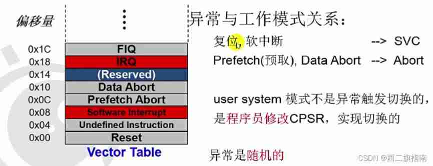
Exception handling of arm
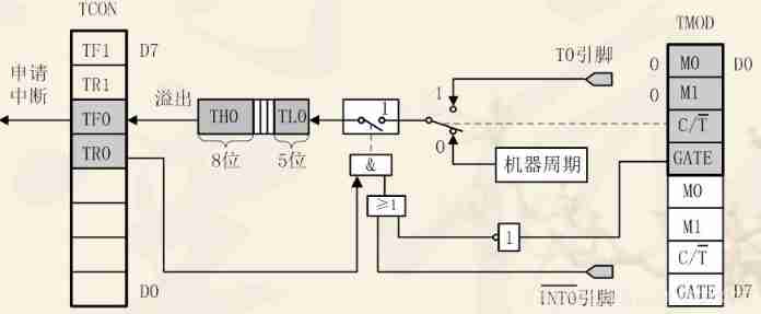
Timer and counter of 51 single chip microcomputer

STM32 interrupt switch

Opencv gray histogram, histogram specification

LeetCode - 673. Number of longest increasing subsequences
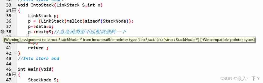
Assignment to '*' form incompatible pointer type 'linkstack' {aka '*'} problem solving

Leetcode interview question 17.20 Continuous median (large top pile + small top pile)

Opencv note 21 frequency domain filtering

Opencv histogram equalization
随机推荐
Blue Bridge Cup for migrant workers majoring in electronic information engineering
LeetCode - 919. Full binary tree inserter (array)
Opencv histogram equalization
The 4G module designed by the charging pile obtains NTP time through mqtt based on 4G network
Stm32f04 clock configuration
openEuler kernel 技術分享 - 第1期 - kdump 基本原理、使用及案例介紹
03 FastJson 解决循环引用
STM32 general timer 1s delay to realize LED flashing
Design of charging pile mqtt transplantation based on 4G EC20 module
My notes on intelligent charging pile development (II): overview of system hardware circuit design
Open Euler Kernel Technology Sharing - Issue 1 - kdump Basic Principles, use and Case Introduction
CV learning notes - edge extraction
Application of external interrupts
2020-08-23
Opencv note 21 frequency domain filtering
byte alignment
Stm32f407 key interrupt
Synchronization control between tasks
Adaptiveavgpool1d internal implementation
Pymssql controls SQL for Chinese queries