Hands on deep learning (36) -- language model and data set

Language models and data sets

   Given such a sequence of text , Language model （language model） The goal is to estimate the joint probability of the sequence .
$$P(x_1,x_2,\dots ,x_T).$$    Language models are very useful . for example , You only need to extract one tag at a time $x_t\sim P(x_t\mid x_{t-1},\dots ,x_1)$, An ideal language model can generate natural text based on the model itself . Unlike monkeys using typewriters , All texts emerging from such a model will be treated as natural language （ for example , English text ） To pass on . Besides , Just based on the text in the previous conversation segment , Enough to generate a meaningful conversation . obviously , We are still far from designing such a system , Because it needs “ understand ” Text , Not just generate grammatically reasonable content .

   For all that , Language models are still very useful , Even in their limited form . for example , The phrase “to recognize speech” and “to wreck a nice beach” It sounds very similar . This similarity will lead to ambiguity in speech recognition , But it's easy to solve it through language model , Because the feeling of the second kind of translation is very strange . Again , In the document summary generation algorithm ,“ Dog bites man ” Than “ Man bites dog ” The frequency is much higher , perhaps “ I want to eat grandma ” Is a rather disturbing statement , and “ I would like to eat , grandma ” Is much kinder .

The application of language model ：

• Make a pre training model （BERT,GPT-3）
• The generation of textual , Given the first few words , Continuous use $x_t\sim p(x_t|x_{t-1})$ To generate subsequent text
• Determine which of the multiple sequences is more common

One 、 Learning language models

1.1 Theoretical explanation

   Obvious , The problem we face is how to manage a document , Even a tag sequence for modeling . Suppose text data is tokenized at the word level , We can rely on the analysis of sequence model in sequence model . Let's start with the basic probability rules ：

Suppose the sequence length is 2, We predict
$$p(x,x^{\prime })=p(x)p(x^{\prime }|x)=\frac{n(x)}{n}\frac{n(x,x^{\prime })}{n(x)}$$

• n Is the total number of words
• n(x),n(x,x’) Is the number of occurrences of a single word and consecutive word pairs

Expand to a length of 3 Under the circumstances ：
$$p(x,x^{\prime },x^{\prime \prime })=p(x)p(x^{\prime }|x)p(x^{\prime \prime }|x,x^{\prime })=\frac{n(x)}{n}\frac{n(x,x^{\prime })}{n(x)}\frac{n(x,x^{\prime },x^{\prime \prime })}{n(x,x^{\prime })}$$

Expand to the case of arbitrary length ：
$$P(x_1,x_2,\dots ,x_T)=\prod _{t=1}^{T}P(x_t\mid x_1,\dots ,x_{t-1}).$$

1.2 Example derivation

for example , It contains four words （deep learning is fun） The probability of a text sequence of is ：

$$P(\text{deep},\text{learning},\text{is},\text{fun})=P(\text{deep})P(\text{learning}\mid \text{deep})P(\text{is}\mid \text{deep},\text{learning})P(\text{fun}\mid \text{deep},\text{learning},\text{is}).$$

   In order to calculate the language model , We need to calculate the probability of a word and the conditional probability of a word after a given first few words . These probabilities are essentially the parameters of the language model .

   here , We assume that the training data set is a large text corpus , such as , All Wikipedia entries , Project Gutenberg , And all the texts published on the Internet . The probability of words in the training data set can be calculated according to the relative word frequency of a given word . for example , The estimated value can be $\hat{P}(\text{deep})$ Calculate as any word “deep” The probability of the first sentence . A slightly less accurate method is to count words “deep” Number of occurrences in the dataset , Then divide it by the total number of words in the whole corpus . This method works well , Especially for frequently occurring words . Next , We can try to estimate

$$\hat{P}(\text{learning}\mid \text{deep})=\frac{n(\text{deep, learning})}{n(\text{deep})},$$

   among $n(x)$ and $n(x,x^{\prime })$ They are the number of occurrences of a single word and consecutive word pairs . Unfortunately , Because continuous word pairs “deep learning” The frequency of occurrence is much lower , So it is much more difficult to estimate the correct probability of such words . especially , For some unusual word combinations , It may not be easy to find enough occurrences to get an accurate estimate . For a combination of three or more words , Things will get worse . Many reasonable combinations of three words may exist , But I can't find it in the dataset . Unless we provide some solution to specify these word combinations as non-zero counts , Otherwise, they cannot be used in the language model . If the data set is small , Or words are very rare , Then the chance of this kind of words appearing once may not be found .

   A common strategy is to perform some form of == Laplacian smoothing (Laplace smoothing)==, The specific method is to add a small constant to all counts . use $n$ Indicates the total number of words in the training set , use $m$ Represents the number of unique words . This solution helps to deal with single element problems , For example, through ：

$$\begin{array}{rl}\hat{P}(x)& =\frac{n(x)+{ϵ}_1/m}{n+{ϵ}_1},\\ \hat{P}(x^{\prime }\mid x)& =\frac{n(x,x^{\prime })+{ϵ}_2\hat{P}(x^{\prime })}{n(x)+{ϵ}_2},\\ \hat{P}(x^{\prime \prime }\mid x,x^{\prime })& =\frac{n(x,x^{\prime },x^{\prime \prime })+{ϵ}_3\hat{P}(x^{\prime \prime })}{n(x,x^{\prime })+{ϵ}_3}.\end{array}$$

among ,${ϵ}_1,{ϵ}_2$ and ${ϵ}_3$ It's a super parameter. . With ${ϵ}_1$ For example ： When ${ϵ}_1=0$ when , Do not apply smoothing ; When ${ϵ}_1$ Near positive infinity ,$\hat{P}(x)$ Near uniform probability distribution $1/m$. The above formula is :cite:Wood.Gasthaus.Archambeau.ea.2011 A fairly primitive variation of other technical implementation methods of .

Unfortunately , A model like this can easily become invalid for the following reasons ：

• First , We need to store all the counts ;
• secondly , This completely ignores the meaning of the word . for example ,“ cat ”（cat） and “ catamount ”（feline） Should appear in the relevant context , But it is quite difficult to adjust these models according to the additional context , However, the language model based on deep learning is very suitable to solve this problem .
• Last , Long word sequences are almost certainly unknown , Therefore, if a model simply counts the frequency of previously seen word sequences , Then the model must be underperforming in the face of this problem .

Two 、 Markov model and $n$ Metagrammar

   Before discussing solutions that involve deep learning , We need to know more concepts and terms . Recall our discussion of Markov models in sequence models , And apply it to language modeling . If $P(x_{t+1}\mid x_t,\dots ,x_1)=P(x_{t+1}\mid x_t)$, Then the distribution on the sequence satisfies the first-order Markov property . The higher the order , The longer the corresponding dependency . This property deduces many approximate formulas that can be applied to sequence modeling ：

$$\begin{array}{rl}P(x_1,x_2,x_3,x_4)& =P(x_1)P(x_2)P(x_3)P(x_4),\\ P(x_1,x_2,x_3,x_4)& =P(x_1)P(x_2\mid x_1)P(x_3\mid x_2)P(x_4\mid x_3),\\ P(x_1,x_2,x_3,x_4)& =P(x_1)P(x_2\mid x_1)P(x_3\mid x_1,x_2)P(x_4\mid x_2,x_3).\end{array}$$

Usually , It involves a 、 The probability formulas for two and three variables are called “ Unary grammar ”（unigram）、“ Binary grammar ”（bigram） and “ Ternary grammar ”（trigram） Model . below , We will learn how to design better models .

3、 ... and 、 Natural language statistics

3.1 Compare multiple grammar groups

   Let's see how it works on real data . Build vocabulary based on time machine data set introduced in text preprocessing , And before printing $10$ The most commonly used （ The most frequent ） word .

import random 
import torch 
from d2l import torch as d2l 

#  Read text data as words
tokens = d2l.tokenize(d2l.read_time_machine())
#  Because each line of text is not necessarily a sentence or a paragraph , So we put all the lines of text together 
corpus = [token for line in tokens for token in line]
vocab = d2l.Vocab(corpus)
vocab.token_freqs[:10]

[('the', 2261),
 ('i', 1267),
 ('and', 1245),
 ('of', 1155),
 ('a', 816),
 ('to', 695),
 ('was', 552),
 ('in', 541),
 ('that', 443),
 ('my', 440)]

#  The most popular words are called stop words 
#  Draw the word frequency diagram of all words , Abscissa is sort , The ordinate is word frequency 
freqs = [freq for token, freq in vocab.token_freqs]
d2l.plot(freqs, xlabel='token: x', ylabel='frequency: n(x)', xscale='log',
         yscale='log')

   Word frequency decays rapidly in a definite way . Eliminate the first few words as exceptions , All the remaining words roughly follow a straight line on the double logarithm graph . This means that the frequency of words meets Zipf's law （Zipf’s law）, That is to say $i$ The frequency of the most commonly used words $n_i$ by ：
$$n_i\propto \frac{1}{i^{\alpha }},$$ Equivalent to
$$\log n_i=-\alpha \log i+c,$$
   among $\alpha$ Is the exponent that characterizes the distribution ,$c$ Is constant . That tells us It is not feasible to model words by counting statistics and smoothing , The result of this modeling will greatly overestimate the frequency of tail words , That is, the so-called uncommon words . But other word combinations , For example, binary grammar 、 Ternary grammar and so on , What will happen ？ Let's see if the frequency of binary grammar and the frequency of unary grammar show the same behavior .

#  The frequency of binary grammar 
#  Will all corpus And remove the first word Of corpus Splicing forms a binary corpus Corpus 
bigram_tokens = [pair for pair in zip(corpus[:-1], corpus[1:])]
bigram_vocab = d2l.Vocab(bigram_tokens)
bigram_vocab.token_freqs[:10]

[(('of', 'the'), 309),
 (('in', 'the'), 169),
 (('i', 'had'), 130),
 (('i', 'was'), 112),
 (('and', 'the'), 109),
 (('the', 'time'), 102),
 (('it', 'was'), 99),
 (('to', 'the'), 85),
 (('as', 'i'), 78),
 (('of', 'a'), 73)]

   It's worth noting here ： Of the ten most frequent word pairs , Nine are made up of two stop words , There is only one with “the time” of . further , Let's see if the frequency of ternary grammar shows the same behavior .

trigram_tokens = [
    triple for triple in zip(corpus[:-2],corpus[1:-1],corpus[2:])
]
trigram_vocab = d2l.Vocab(trigram_tokens)
trigram_vocab.token_freqs[:10]

[(('the', 'time', 'traveller'), 59),
 (('the', 'time', 'machine'), 30),
 (('the', 'medical', 'man'), 24),
 (('it', 'seemed', 'to'), 16),
 (('it', 'was', 'a'), 15),
 (('here', 'and', 'there'), 15),
 (('seemed', 'to', 'me'), 14),
 (('i', 'did', 'not'), 14),
 (('i', 'saw', 'the'), 13),
 (('i', 'began', 'to'), 13)]

#  Of the three models frequency Draw it out 
bigram_freqs = [freq for token, freq in bigram_vocab.token_freqs]
trigram_freqs = [freq for token, freq in trigram_vocab.token_freqs]
d2l.plot([freqs, bigram_freqs, trigram_freqs], xlabel='token: x',
         ylabel='frequency: n(x)', xscale='log', yscale='log',
         legend=['unigram', 'bigram', 'trigram'])

The above picture has many key points

1. Except for monogrammatical words , Word sequences also follow Zipf's law , Even though the formula $n_i\propto \frac{1}{i^{\alpha }},$ Medium i The index is smaller （ The size of the index is affected by the length of the sequence ）
2. In Glossary n The number of tuples is not that large , There are quite a lot of structures in presentation languages
3. quite a lot n Tuples rarely appear , Making Laplacian smoothing unsuitable for language models

3.2 Read long sequence data

   Because sequence data is continuous in nature , Therefore, we need to solve this problem when processing data . In the sequence model, we do this in a quite special way . When the sequence becomes too long to be processed all at once by the model , We may want to split such a sequence to facilitate model reading . Now let's describe the overall strategy . Before introducing the model , Suppose we will use neural networks to train language models , The network processing in the model has a predefined length （ for example $n$ Time steps ） A small batch sequence of . The problem now is how to randomly generate the characteristics and labels of a small batch of data for reading .

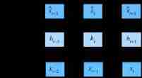
   First , Because the text sequence can be arbitrarily long , For example, the whole book 《 Time machine 》(The Time Machine), Therefore, any long sequence can be divided into subsequences with the same number of time steps . When training our neural networks , Such a small batch of quantum sequences will be input into the model . Suppose that the network only deals with $n$ A subsequence of time steps . The following figure shows all the different ways to obtain subsequences from the original text sequence , among $n=5$, And the mark of each time step corresponds to a character . Please note that , Because we can choose any offset to indicate the initial position , So we have a lot of freedom .

   therefore , Which one should we choose ？ in fact , They are all equally good . However , If we only choose one offset , So what is used to train the network 、 The coverage of all possible subsequences will be limited . therefore , We can divide the sequence from the random offset , At the same time Coverage （coverage） and Randomness （randomness）. below , We will describe how to implement Random sampling （random sampling） and Sequential partition （sequential partitioning） Strategy .

3.2.1 Random sampling

   In random sampling , Each sample is a subsequence arbitrarily captured on the original long sequence . In the iteration process , From two adjacent 、 Random 、 Subsequences in a small batch are not necessarily adjacent to the original sequence . For language modeling , The goal is to predict the next marker based on the markers we have seen so far , Therefore, the tag is the original sequence shifted by a tag .

   The following code generates a small batch randomly from the data every time . ad locum , Parameters batch_size Specifies the number of neutron sequence samples per small batch , Parameters num_steps Is the number of predefined time steps in each subsequence .

def seq_data_iter_random(corpus,batch_size,num_steps):
    """ Use random sampling to generate a small batch of quantum sequences """
    #  The sequence is partitioned from a random offset , The random range includes `num_steps - 1`
    corpus = corpus[random.randint(0, num_steps - 1):]
    #  subtract 1, Because we need to consider labels 
    num_subseqs = (len(corpus) - 1) // num_steps
    #  The length is `num_steps` The starting index of the subsequence of 
    initial_indices = list(range(0, num_subseqs * num_steps, num_steps))
    #  In the iterative process of random sampling ,
    #  From two adjacent 、 Random 、 Subsequences in a small batch are not necessarily adjacent to the original sequence 
    random.shuffle(initial_indices)

    def data(pos):
        #  Return from `pos` The length at the beginning of the position is `num_steps` Sequence 
        return corpus[pos:pos + num_steps]

    num_batches = num_subseqs // batch_size
    for i in range(0, batch_size * num_batches, batch_size):
        #  ad locum ,`initial_indices` Random start index containing subsequences 
        initial_indices_per_batch = initial_indices[i:i + batch_size]
        X = [data(j) for j in initial_indices_per_batch]
        Y = [data(j + 1) for j in initial_indices_per_batch]
        yield torch.tensor(X), torch.tensor(Y)

   Let's generate an example from $0$ To $34$ Sequence . Suppose the batch size is $2$ , The number of time steps is $5$, This means that you can generate $\lfloor (35-1)/5\rfloor =6$ individual “ features － label ” Subsequence pair . Set the small batch size to $2$ when , We can only get $3$ A small batch .

my_seq = list(range(35))
for X, Y in seq_data_iter_random(my_seq, batch_size=2, num_steps=5):
    print('X: ', X, '\nY:', Y)

[3, 4, 5, 6, 7, 8, 9, 10, 11, 12, 13, 14, 15, 16, 17, 18, 19, 20, 21, 22, 23, 24, 25, 26, 27, 28, 29, 30, 31, 32, 33, 34]
[0, 5, 10, 15, 20, 25]
X:  tensor([[18, 19, 20, 21, 22],
        [28, 29, 30, 31, 32]]) 
Y: tensor([[19, 20, 21, 22, 23],
        [29, 30, 31, 32, 33]])
X:  tensor([[ 8,  9, 10, 11, 12],
        [ 3,  4,  5,  6,  7]]) 
Y: tensor([[ 9, 10, 11, 12, 13],
        [ 4,  5,  6,  7,  8]])
X:  tensor([[23, 24, 25, 26, 27],
        [13, 14, 15, 16, 17]]) 
Y: tensor([[24, 25, 26, 27, 28],
        [14, 15, 16, 17, 18]])

3.2.2 Sequential partition

Ensure that the subsequences in two adjacent small batches are also adjacent to the original sequence （ In the iteration process based on small batch, the order of split subsequences is also preserved ）

def seq_data_iter_sequential(corpus,batch_size,num_steps):
    """ Use sequential partitioning to generate a small batch of quantum sequences """
    #  Divide the sequence from the random offset 
    offset = random.randint(0,num_steps)
    num_tokens = ((len(corpus)- offset -1)//batch_size)*batch_size
    Xs = torch.tensor(corpus[offset:offset+num_tokens])
    Ys = torch.tensor(corpus[offset+1:offset+num_tokens+1])
    Xs,Ys = Xs.reshape(batch_size,-1),Ys.reshape(batch_size,-1)
    num_batches = Xs.shape[1]//num_steps
    for i in range(0,num_steps*num_batches,num_steps):
        X = Xs[:,i:i+num_steps]
        Y = Ys[:,i:i+num_steps]
        yield X,Y

for X, Y in seq_data_iter_sequential(my_seq, batch_size=2, num_steps=5):
    print('X: ', X, '\nY:', Y)

X:  tensor([[ 0,  1,  2,  3,  4],
        [17, 18, 19, 20, 21]]) 
Y: tensor([[ 1,  2,  3,  4,  5],
        [18, 19, 20, 21, 22]])
X:  tensor([[ 5,  6,  7,  8,  9],
        [22, 23, 24, 25, 26]]) 
Y: tensor([[ 6,  7,  8,  9, 10],
        [23, 24, 25, 26, 27]])
X:  tensor([[10, 11, 12, 13, 14],
        [27, 28, 29, 30, 31]]) 
Y: tensor([[11, 12, 13, 14, 15],
        [28, 29, 30, 31, 32]])

3.2.3 Collate sampling function

class SeqDataLoader:  #@save
    """ An iterator that loads sequence data ."""
    def __init__(self, batch_size, num_steps, use_random_iter, max_tokens):
        if use_random_iter:
            self.data_iter_fn = d2l.seq_data_iter_random
        else:
            self.data_iter_fn = d2l.seq_data_iter_sequential
        self.corpus, self.vocab = d2l.load_corpus_time_machine(max_tokens)
        self.batch_size, self.num_steps = batch_size, num_steps

    def __iter__(self):
        return self.data_iter_fn(self.corpus, self.batch_size, self.num_steps)

#  Defined function load_data_time_machine Return both data iterators and vocabularies 
def load_data_time_machine(batch_size, num_steps,  #@save
                           use_random_iter=False, max_tokens=10000):
    """ Returns the iterator and vocabulary of the time machine dataset ."""
    data_iter = SeqDataLoader(batch_size, num_steps, use_random_iter,
                              max_tokens)
    return data_iter, data_iter.vocab

Four 、 Arrangement

• Language model is the key of natural language processing
• n Metagrammar , By truncating the Correlation , It provides a practical model for dealing with long sequences
• There is a problem with long sequences ： Rarely or never
• Zipf's law governs the distribution of words , It's not just monadic grammar , For the rest n Metagrammar also applies
• Laplacian smoothing can effectively deal with phrases composed of low-frequency words with rich structure and insufficient frequency
• The main ways to read long sequences are random sampling and sequential partitioning . In the iteration process , The latter can ensure that subsequences from two adjacent small batches are also adjacent to the original sequence .

5、 ... and 、 practice

1. Suppose there is $100,000$ Word . How many word frequencies and adjacent multi word frequencies need to be stored in a quaternion grammar ？
   I think word frequency is $10^4$, And the adjacent multi word frequency I think is $10^5\ast 10^5\ast 10^5\ast 10^5=(10^5{)}^4$

2. How do we model a series of conversations ？
   I'm not in this direction , Post some thoughts of others
   https://zhuanlan.zhihu.com/p/296331236

3. Unary grammar 、 The exponent of Zipf's law of binary grammar and ternary grammar is different , Can you try to estimate ？

4. Think about other ways to read long sequence data ？
   I'm daydreaming ：

   • For long sequences, in addition to cutting methods , Is it possible to save all the sequence lengths directly , And then random one seed Select the sampling location , Then continuously random sampling , If the sampling has a uniform probability distribution , In theory, each word The probability of being selected is the same . In fact, such sampling is feasible to a certain extent .
   • Except for forward cutting , Reverse can also cut

5. Consider the random offset we use to read long sequences .

   1. Why random offsets are a good idea ？
      While reducing the frequency of continuous words, it ensures the possibility of using each word
   2. Will it really achieve perfect uniform distribution on the sequence of documents ？
      Can't , Because of the influence of random numbers
   3. What can you do to make the distribution more uniform ？
      Reverse and re offset the sampling ？

6. If we want a sequence sample to be a complete sentence , So what problems will this bring in small batch sampling ？ How to solve ？