ML11-SKlearn实现支持向量机

SKlearn库 实现 SVM

%matplotlib inline 
#为了在notebook中画图展示
import numpy as np
import matplotlib.pyplot as plt
from scipy import stats
import seaborn as sns; sns.set()

#随机来点数据，使用sklearn下的方法随机生成数据点
#其中 cluster_std是数据的离散程度
from sklearn.datasets.samples_generator import make_blobs
X, y = make_blobs(n_samples=50, centers=2,
                  random_state=0, cluster_std=0.60)
plt.scatter(X[:, 0], X[:, 1], c=y, s=50, cmap='autumn')

训练一个基本的SVM

#分类任务
from sklearn.svm import SVC 
#线性核函数 相当于不对数据进行变换
model = SVC(kernel='linear')
model.fit(X, y)

绘图函数的模板

#绘图函数
def plot_svc_decision_function(model, ax=None, plot_support=True):
   
    if ax is None:
        ax = plt.gca()
    xlim = ax.get_xlim()
    ylim = ax.get_ylim()
    
    # 用SVM自带的decision_function函数来绘制
    x = np.linspace(xlim[0], xlim[1], 30)
    y = np.linspace(ylim[0], ylim[1], 30)
    Y, X = np.meshgrid(y, x)
    xy = np.vstack([X.ravel(), Y.ravel()]).T
    P = model.decision_function(xy).reshape(X.shape)
    
    # 绘制决策边界
    ax.contour(X, Y, P, colors='k',
               levels=[-1, 0, 1], alpha=0.5,
               linestyles=['--', '-', '--'])
    
    # 绘制支持向量
    if plot_support:
        ax.scatter(model.support_vectors_[:, 0],
                   model.support_vectors_[:, 1],
                   s=300, linewidth=1, alpha=0.2);
    ax.set_xlim(xlim)
    ax.set_ylim(ylim)

plt.scatter(X[:, 0], X[:, 1], c=y, s=50, cmap='autumn')
plot_svc_decision_function(model)

这条线就是我们希望得到的决策边界啦

观察发现有3个点做了特殊的标记，它们恰好都是边界上的点

它们就是我们的support vectors（支持向量）

在Scikit-Learn中, 它们存储在这个位置 support_vectors_（一个属性）

观察可以发现，只需要支持向量我们就可以把模型构建出来

接下来我们尝试一下，用不同多的数据点，看看效果会不会发生变化

分别使用60个和120个数据点

def plot_svm(N=10, ax=None):
    X, y = make_blobs(n_samples=200, centers=2,
                      random_state=0, cluster_std=0.60)
    X = X[:N]
    y = y[:N]
    model = SVC(kernel='linear', C=1E10)
    model.fit(X, y)
    
    ax = ax or plt.gca()
    ax.scatter(X[:, 0], X[:, 1], c=y, s=50, cmap='autumn')
    ax.set_xlim(-1, 4)
    ax.set_ylim(-1, 6)
    plot_svc_decision_function(model, ax)
# 分别对不同的数据点进行绘制
fig, ax = plt.subplots(1, 2, figsize=(16, 6))
fig.subplots_adjust(left=0.0625, right=0.95, wspace=0.1)
for axi, N in zip(ax, [60, 120]):
    plot_svm(N, axi)
    axi.set_title('N = {0}'.format(N))

引入核函数的SVM

绘制另一种数据集分布

from sklearn.datasets.samples_generator import make_circles
# 绘制另外一种数据集
X, y = make_circles(100, factor=.1, noise=.1)
#看看这回线性和函数能解决嘛
clf = SVC(kernel='linear').fit(X, y)

plt.scatter(X[:, 0], X[:, 1], c=y, s=50, cmap='autumn')
plot_svc_decision_function(clf, plot_support=False);

#加入了新的维度r
from mpl_toolkits import mplot3d
r = np.exp(-(X ** 2).sum(1))
# 可以想象一下在三维中把环形数据集进行上下拉伸
def plot_3D(elev=30, azim=30, X=X, y=y):
    ax = plt.subplot(projection='3d')
    ax.scatter3D(X[:, 0], X[:, 1], r, c=y, s=50, cmap='autumn')
    ax.view_init(elev=elev, azim=azim)
    ax.set_xlabel('x')
    ax.set_ylabel('y')
    ax.set_zlabel('r')

plot_3D(elev=45, azim=45, X=X, y=y)

#加入高斯核函数
clf = SVC(kernel='rbf')
clf.fit(X, y)

#这回厉害了！
plt.scatter(X[:, 0], X[:, 1], c=y, s=50, cmap='autumn')
plot_svc_decision_function(clf)
plt.scatter(clf.support_vectors_[:, 0], clf.support_vectors_[:, 1],
            s=300, lw=1, facecolors='none');

调节SVM参数

# 这份数据集中cluster_std稍微大一些，这样才能体现出软间隔的作用
X, y = make_blobs(n_samples=100, centers=2,
                  random_state=0, cluster_std=0.8)
plt.scatter(X[:, 0], X[:, 1], c=y, s=50, cmap='autumn')

C参数

#加大游戏难度的数据集
X, y = make_blobs(n_samples=100, centers=2,
                  random_state=0, cluster_std=0.8)

fig, ax = plt.subplots(1, 2, figsize=(16, 6))
fig.subplots_adjust(left=0.0625, right=0.95, wspace=0.1)
# 选择两个C参数来进行对别实验，分别为10和0.1
for axi, C in zip(ax, [10.0, 0.1]):
    model = SVC(kernel='linear', C=C).fit(X, y)
    axi.scatter(X[:, 0], X[:, 1], c=y, s=50, cmap='autumn')
    plot_svc_decision_function(model, axi)
    axi.scatter(model.support_vectors_[:, 0],
                model.support_vectors_[:, 1],
                s=300, lw=1, facecolors='none');
    axi.set_title('C = {0:.1f}'.format(C), size=14)

噶玛参数，越大映射的维度越高，模型越复杂。

X, y = make_blobs(n_samples=100, centers=2,
                  random_state=0, cluster_std=1.1)

fig, ax = plt.subplots(1, 2, figsize=(16, 6))
fig.subplots_adjust(left=0.0625, right=0.95, wspace=0.1)
# 选择不同的gamma值来观察建模效果
for axi, gamma in zip(ax, [10.0, 0.1]):
    model = SVC(kernel='rbf', gamma=gamma).fit(X, y)
    axi.scatter(X[:, 0], X[:, 1], c=y, s=50, cmap='autumn')
    plot_svc_decision_function(model, axi)
    axi.scatter(model.support_vectors_[:, 0],
                model.support_vectors_[:, 1],
                s=300, lw=1, facecolors='none');
    axi.set_title('gamma = {0:.1f}'.format(gamma), size=14)

对于比较大的噶玛值，边界分的很清晰，但是泛化能力比较低；偏小的噶玛值，分错了一些数据点，但是泛化能力强，更加有使用价值。

人脸识别实例

#读取数据集
from sklearn.datasets import fetch_lfw_people
#每个人的人脸至少有60个
faces = fetch_lfw_people(min_faces_per_person=60)
#看一下数据的规模
print(faces.target_names)
print(faces.images.shape)

# 3行5列的布局
fig, ax = plt.subplots(3, 5)
for i, axi in enumerate(ax.flat):
    axi.imshow(faces.images[i], cmap='bone')
    axi.set(xticks=[], yticks=[],
            xlabel=faces.target_names[faces.target[i]])

from sklearn.svm import SVC
from sklearn.decomposition import PCA
from sklearn.pipeline import make_pipeline

#降维到150维
pca = PCA(n_components=150, whiten=True, random_state=42)
svc = SVC(kernel='rbf', class_weight='balanced')
#先降维然后再SVM
model = make_pipeline(pca, svc)

划分数据集

from sklearn.model_selection import train_test_split
Xtrain, Xtest, ytrain, ytest = train_test_split(faces.data, faces.target,
                                                random_state=40)

使用grid search cross-validation来选择我们的参数，遍历C和噶玛，看看哪个效果好。

from sklearn.model_selection import GridSearchCV
param_grid = {
    'svc__C': [1, 5, 10],
              'svc__gamma': [0.0001, 0.0005, 0.001]}
grid = GridSearchCV(model, param_grid)

%time grid.fit(Xtrain, ytrain)
print(grid.best_params_)

选好后用我们的模型来做预测。

model = grid.best_estimator_
yfit = model.predict(Xtest)
yfit.shape

结果展示

fig, ax = plt.subplots(4, 6)
for i, axi in enumerate(ax.flat):
    axi.imshow(Xtest[i].reshape(62, 47), cmap='bone')
    axi.set(xticks=[], yticks=[])
    axi.set_ylabel(faces.target_names[yfit[i]].split()[-1],
                   color='black' if yfit[i] == ytest[i] else 'red')
fig.suptitle('Predicted Names; Incorrect Labels in Red', size=14);

from sklearn.metrics import classification_report
print(classification_report(ytest, yfit,
                            target_names=faces.target_names))

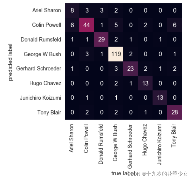
精度值和召回率

混淆矩阵

from sklearn.metrics import confusion_matrix
mat = confusion_matrix(ytest, yfit)
sns.heatmap(mat.T, square=True, annot=True, fmt='d', cbar=False,
            xticklabels=faces.target_names,
            yticklabels=faces.target_names)
plt.xlabel('true label')
plt.ylabel('predicted label');