Matlab digital image processing experiment 2: single pixel spatial image enhancement

One 、 The experiment purpose

1、 Familiar with single pixel spatial image enhancement methods , Understand and master histogram equalization and normalization to realize image enhancement

Two 、 Experimental environment

Matlab 2020B

3、 ... and 、 Experimental content

subject

1） For an image with low contrast resolution, the gray level transformation method other than histogram processing method is used to realize image enhancement .（ Figure optional ）
2） Histogram equalization and normalization methods are used for an image with low contrast resolution （ Single mapping or group mapping ） Realize image enhancement , The system function and the function written by ourselves are used to realize the application function .（ Figure optional ）
3） Write the experiment report . Reporting requirements ： The experiment purpose 、 Experimental content 、 Experimental process 、 Experimental summary and more detailed graphic description .

Related knowledge

For low resolution images , We can use the method based on spatial image enhancement . In addition to histogram processing , You can also use gray inversion 、 Logarithmic transformation 、 Exponential transformation 、 Contrast stretch 、 Gray slice, etc .
Use exponential transformation , Use the formula for each pixel $s=c{r}^{\gamma }$, among $c$ Is constant and $c=1$,$\gamma$ Is the parameter ,$\gamma >1$ The image darkens when ,$\gamma <1$ Image lightens when ,$r$ Is the gray value in the original image , The value range is $r\in [0,1]$,$s$ Is the gray value in the new image , if $s>1$ Then take $s=1$.
The implementation of gray inversion is relatively simple . Use the formula for each pixel $s=L-1-r$.$L$ Is the gray level , stay uint8 In the image of ,$L=256$.$r$ Is the gray value in the original image ,$s$ Is the gray value in the new image .
When using logarithmic transformation , Use the formula $s=c\log (r+1)$, among $c$ Is a parameter and $c$ It's OK not to 1,$r$ Is the gray value in the original image and $r\ge 0$.
Contrast stretching can be used matlab Self contained function imadjust Realization ,imadjust Can take three parameters , They are the original drawings 、 The range of gray values entered 、 Range of output gray value . You can also write functions to realize . In this experiment , Use linear transformation to achieve the effect of contrast stretching . Take the gray value of the lowest gray value in the original image as $a_0$, take $b_0=0.5$. Take the minimum new gray value as $a_{new}$, The maximum new gray value is $b_{new}$. Then for each pixel ,$s=a_{new}+\frac{b_{new}-a_{new}}{b_0-a_0}\ast (r-a_0)$. among ,$r$ Is the gray value in the original image and $0\le r\le 1$,$s$ Is the gray value in the new image and $0\le s\le 1$. For the calculation results $\le 0$ The point of needs to be set to 0, For the calculation results $\ge 1$ The point of needs to be set to 1.
Histogram equalization can be used matlab Self contained function histeq Realization ,histeq With two parameters , They are the original drawings 、 Gray level series of image . call imhist function , You can also get and output the histogram of the image . You can also write functions to realize .
When writing a function to realize histogram equalization , First, process the histogram of the original image . remember $h(r_k)=n_k$,$r_k$ Is a certain gray level in the original image ,$n_k$ The gray level in the image is the same as $r_k$ The number of pixels . take $p(r_k)=\frac{h(r_k)}{n}=\frac{n_k}{n}$, among $n$ Is the total number of pixels in the figure , be $p(r_k)$ It's grayscale $r_k$ The probability density of the probability of occurrence . For the first $k$ Gray scale ,$s_k=T(r_k)={\sum }_{j=0}^k{p}_r(r_j)={\sum }_{j=0}^k\frac{n_j}{n}$ Is its cumulative distribution function . Next , Deal with the second $k$ The gray level mapped in the new image $S(k)=\mathrm{int}[(\max (r_k)-\min (r_k))\ast s_k+0.5]$. Last , Map the gray level of each pixel in the original image to the gray level of the corresponding pixel in the new image .
Histogram matching （ Prescriptive ） Also used histeq Realization .histeq The two parameters of are the original graph 、 Histogram of the matched image .
Realizing histogram specification in writing functions （ Histogram matching ） when , alike , First, the histogram of the original image and the histogram of the matched image are processed . Histogram matching can be achieved by single mapping , You can also use group mapping to implement . When implementing single mapping , The corresponding gray value in the original image is mapped into the gray value corresponding to the cumulative probability density of the matched image according to the cumulative probability density . When implementing group mapping , The corresponding gray value of the matched image is mapped into the corresponding gray value of the original image according to the cumulative probability density , And need to fill the gap .

Part of the core code

I_0=imread("Couple.bmp");
I_0=im2double(I_0);
c=1;
gamma=0.40;
[w,h]=size(I_0);
I_1=zeros(w,h);
for i=1:w
    for j=1:h
        I_1(i,j)=I_0(i,j).^gamma;
    end
end
title(" experiment 1-1")
subplot(1,2,1);imshow(I_0);title(' Original picture ')
subplot(1,2,2);imshow(I_1);title(' New graph ')

Completed the exponential transformation , Using the formula $s=c{r}^{\gamma }$,$\gamma =0.4$, Success makes the image brighter .

I_0=imread("Couple.bmp");
I_0=im2double(I_0);
c=1;
gamma=0.40;
[w,h]=size(I_0);
I_1=imadjust(I_0,[0.1 0.5],[0 1]);
title(" experiment 2-3")
subplot(1,2,1);imshow(I_0);title(' Original picture ')
subplot(1,2,2);imshow(I_1);title('imadjust')

Finished the contrast stretching of the image , Use matlab Self contained imadjust Function implementation , Make the image bright .

I=im2double(I);
anew=0;
bnew=1;
a0=min(min(min(I)));
b0=0.5;
A1=anew+(bnew-anew)/(b0-a0)*(I-a0);
[row,col]=size(I);
for i=1:row
    for j=1:col
        if(A1(i,j)<0)
            A1(i,j)=0;
        end
        if A1(i,j)>1
            A1(i,j)=1;
        end
    end
end
imshow(A1)

Finished the contrast stretching of the image , Use self written program to realize . The minimum new gray value is $a_{new}$, The maximum new gray value is $b_{new}$. Then for each pixel ,$s=a_{new}+\frac{b_{new}-a_{new}}{b_0-a_0}\ast (r-a_0)$. Last , Handle $s>1$ or $s<0$ The situation of .

I_0=imread("Couple.bmp");
I_0=im2double(I_0);
c=2;
[w,h]=size(I_0);
I_1=zeros(w,h);
for i=1:w
    for j=1:h
        I_1(i,j)=c*log(I_0(i,j)+1);
    end
end
title(" experiment 1-1")
subplot(1,2,1);imshow(I_0);title(' Original picture ')
subplot(1,2,2);imshow(I_1);title(' New graph ')

Completed the logarithmic transformation of the image , take $c=2$, Successfully brighten the image .

I=imread("Couple.bmp");
I=im2double(I);
subplot(1,2,1);imshow(I);title(' Original picture ')
[w,h]=size(I);
I1=ones(w,h);
for i=1:w
    for j=1:h
        I1(i,j)=1-I(i,j);
    end
end
subplot(1,2,2);imshow(I1);title(' New graph ')

Completed the gray inversion of the image , Make the dark place bright , The light turns dark .

I=imread("Couple.bmp");
subplot(2,2,1)
imshow(I);title(" Original picture ")
subplot(2,2,2)
imhist(I);title(" Original histogram ")
ylim('auto')
g=histeq(I,256);
subplot(2,2,3)
imshow(g);title(" New graph ")
subplot(2,2,4)
imhist(g);title(" New histogram ")
ylim('auto')

Call system functions to realize histogram equalization

I=imread("Couple.bmp");
histogram=zeros(1,255);
[w,h]=size(I);
for i=1:w
    for j=1:h
        histogram(I(i,j)+1)=histogram(I(i,j)+1)+1;% Process the number of pixels of each gray level 
    end
end
%bar(zhifangtu)
n=w*h;% The total number of pixels on the graph 
p=histogram/n;% Probability density function 
s=zeros(1,255);% Cumulative probability density 
s(1)=p(1);
for i=2:255
    s(i)=s(i-1)+p(i);
end
newimg=zeros(w,h);% New graph 
for i=1:w
    for j=1:h
        newimg(i,j)=s(I(i,j)+1);% The corresponding pixel value of the new image is the corresponding pixel value of the original image * Gray scale . But in this code , Use double Save map 
    end
end
imshow(newimg)
newimg=im2uint8(newimg);
newhistogram=zeros(1,255);
for i=1:w
    for j=1:h
        newhistogram(newimg(i,j)+1)=newhistogram(newimg(i,j)+1)+1;% The number of pixels of each gray level in the new image 
    end
end
title(" experiment 2-8")
subplot(2,2,1);imshow(I);title(' Original picture ')
subplot(2,2,2);bar(histogram);title(' Original histogram ')
subplot(2,2,3);imshow(newimg);title(' Image after histogram equalization ')
subplot(2,2,4);bar(newhistogram);title(' Histogram after histogram equalization ')

Write a function to realize the histogram equalization of the image . First process the probability density of each gray level of the original image , Then solve each gray level

I=imread("Couple.bmp");
Imatch=imread("match.png");
Imatch=rgb2gray(Imatch);
[histogram,x]=imhist(Imatch);
Inew=histeq(I,histogram);
subplot(3,2,1),imshow(I);title(" Original picture ")
subplot(3,2,2);imhist(I);title(" Original histogram ")
subplot(3,2,3);imshow(Imatch);title(" Matched graph ")
subplot(3,2,4);imhist(Imatch);title(" Matched histogram ")
subplot(3,2,5);imshow(Inew);title(" New graph ")
subplot(3,2,6);imhist(Inew);title(" New histogram ")

Use matlab The built-in function realizes histogram matching （ Histogram specification ）.

I=imread("Couple.bmp");
histogram=zeros(1,255);
[w,h]=size(I);
for i=1:w
    for j=1:h
        histogram(I(i,j)+1)=histogram(I(i,j)+1)+1;% Process the number of pixels of each gray level 
    end
end
%bar(zhifangtu)
n=w*h;
p=histogram/n;
s1=zeros(1,255);
s1(1)=p(1);
for i=2:255
    s1(i)=s1(i-1)+p(i);
end
I2=imread("match.png");% Matched image 
histogram2=zeros(1,255);
I2=im2gray(I2);
[w2,h2]=size(I2);
for i=1:w2
    for j=1:h2
        histogram2(I2(i,j)+1)=histogram2(I2(i,j)+1)+1;% Process the number of pixels of each gray level 
    end
end
n2=w2*h2;
p2=histogram2/n2;
s2=zeros(1,255);
s2(1)=p2(1);
for i=2:255
    s2(i)=s2(i-1)+p2(i);
end
map=zeros(1,255);% Set gray level i mapping j
for i=1:255
    for j=1:254
        if (s1(i)>=s2(j) && s1(i)<=s2(j+1))% Match the gray level of the original image with that of the new image 
            if (abs(s1(i)-s2(j))<abs(s1(i)-s2(j+1)))% Match to the closest point of probability density 
                map(i)=j;
            else
                map(i)=j+1;
            end
            break
        end
    end
end
newimg=zeros(w,h);% New graph 
for i=1:w
    for j=1:h
        newimg(i,j)=map(I(i,j)+1);% Map the pixels of the original image to the new image according to the matching relationship 
    end
end
newimg=newimg/255;
newimg=im2uint8(newimg);
newhistogram=zeros(1,255);
for i=1:w
    for j=1:h
        newhistogram(newimg(i,j)+1)=newhistogram(newimg(i,j)+1)+1;% Histogram of new graph 
    end
end
subplot(3,2,1),imshow(I);title(" Original picture ")
subplot(3,2,2);bar(histogram);title(" Original histogram ")
subplot(3,2,3);imshow(Imatch);title(" Matched graph ")
subplot(3,2,4);bar(histogram2);title(" Matched histogram ")
subplot(3,2,5);imshow(newimg);title(" New graph ")
subplot(3,2,6);bar(newhistogram);title(" New histogram ")

Write a function to realize histogram matching , Realize single mapping . First, the probability density and cumulative probability density of each gray level of the original image are processed , Then process the probability density and cumulative probability density of each gray level of the matched image . Last , The gray level of the original image is mapped into the gray level of the matched image according to the cumulative probability density . Get the relationship between the gray level of the original image and the gray level it is mapped into , Create a new image and fill in the mapping value of the gray level of the corresponding pixel of the original image .

I=imread("Couple.bmp");
histogram=zeros(1,255);
[w,h]=size(I);
for i=1:w
    for j=1:h
        histogram(I(i,j)+1)=histogram(I(i,j)+1)+1;% Process the number of pixels of each gray level 
    end
end
%bar(zhifangtu)
n=w*h;
p=histogram/n;
s1=zeros(1,255);
s1(1)=p(1);
for i=2:255
    s1(i)=s1(i-1)+p(i);
end
 
I2=imread("match.png");% Matched image 
histogram2=zeros(1,255);
I2=im2gray(I2);
[w2,h2]=size(I2);
for i=1:w2
    for j=1:h2
        histogram2(I2(i,j)+1)=histogram2(I2(i,j)+1)+1;% Process the number of pixels of each gray level 
    end
end
n2=w2*h2;
p2=histogram2/n2;
s2=zeros(1,255);
s2(1)=p2(1);
for i=2:255
    s2(i)=s2(i-1)+p2(i);
end
map=zeros(1,255);% Set gray level i mapping j
for j=1:255
    for i=1:254
        if (s2(j)>=s1(i) && s2(j)<=s1(i+1))% Map the gray level of the new image to the gray level of the original image , Group mapping 
            if (abs(s2(j)-s1(i))<abs(s2(j)-s1(i+1)))
                map(i)=j;
            else
                map(i)=j+1;
            end
            break
        end
    end
end
for i=2:255
    if (map(i)==0)
        map(i)=map(i-1);
    end
end
 
newimg=zeros(w,h);
for i=1:w
    for j=1:h
        newimg(i,j)=map(I(i,j)+1);
    end
end
newimg=newimg/255;
newimg=im2uint8(newimg);
newhistogram=zeros(1,255);
for i=1:w
    for j=1:h
        newhistogram(newimg(i,j)+1)=newhistogram(newimg(i,j)+1)+1;
    end
end
subplot(3,2,1),imshow(I);title(" Original picture ")
subplot(3,2,2);bar(histogram);title(" Original histogram ")
subplot(3,2,3);imshow(Imatch);title(" Matched graph ")
subplot(3,2,4);bar(histogram2);title(" Matched histogram ")
subplot(3,2,5);imshow(newimg);title(" New graph ")
subplot(3,2,6);bar(newhistogram);title(" New histogram ")

Write a function to realize histogram matching , Realized group mapping . alike , First, the probability density and cumulative probability density of each gray level of the original image are processed , Then process the probability density and cumulative probability density of each gray level of the matched image . The matched gray level is mapped into the gray level of the original image according to the cumulative probability density . after , If there is a missing value , That is, the gray level of the new image mapped to a certain gray level in the original image is unknown , You need to fill in the missing value . Get the relationship between the gray level of the original image and the gray level it is mapped into , Create a new image and fill in the mapping value of the gray level of the corresponding pixel of the original image .

experimental result

The exponential transformation is successfully realized , You can see that the new image is significantly brighter than the original 、 Higher contrast , because $s=c{r}^{\gamma }$ Of $\gamma <1$.

Successfully achieved contrast stretching , Use matlab Self contained imadjust function . Due to the selection of parameters , You can see , Some points are obviously brighter , And the color of some pixels remains unchanged .

Realize logarithmic transformation , Take parameters $c>1$. You can clearly see that some of the points are bright .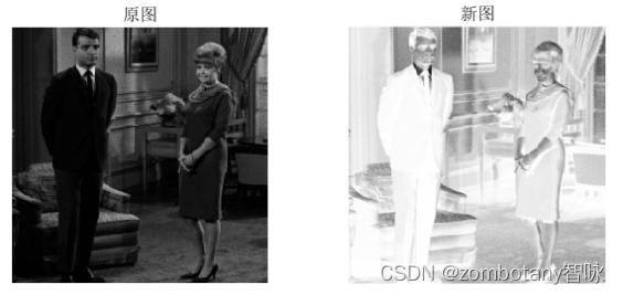

Realize gray inversion .

Writing functions to implement functions similar to imadjust The effect of , take $[0,0.5]$ The gray value of is mapped to $[0,1]$. It is obvious that the image is brightened .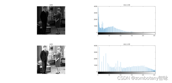

Use the histogram equalization function provided by the system , Histogram equalization is realized . You can see , The image is significantly brighter . The gray value of the original image is distributed around 0_{150 Within the scope of , After being equalized by histogram , Gray value distribution is more “ equilibrium ” 了 , Distribution in 0}255 The scope of the . Compared with the previous transformation that is not based on histogram , This method better saves some details of the image , It looks more natural 、 real .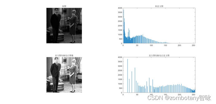

Use self written programs , Histogram equalization is realized . You can see , The program written by myself well restores the implementation effect of the histogram equalization program of the system . It is not only similar to the processing result of the system's own function on the image , And this can be reflected in the histogram image .

Called the system's own function , Achieve histogram matching . You can see , The matched histogram is in 200~230 There is an obvious peak in the distribution of gray level , So this peak is also reflected in the image after histogram matching , Also in the 200~230 There is a peak on the gray level . therefore , The picture is obviously brighter . however , Because it is too bright selected by the matching graph , So the new picture is too bright .

Histogram matching is realized by ourselves , Using the method of single mapping . You can see , In terms of the overall effect of processing, it restores the effect of the function of the system .

Histogram matching is realized by ourselves , Using the method of group mapping . Although the program that implements group mapping is slightly different from the program that implements single mapping , But the effect is similar , All roads lead to Rome , It is similar to the effect of calling the function of the system .

Four 、 Summary of experiments