当前位置:网站首页>In depth description of Weibull distribution (1) principle and formula
In depth description of Weibull distribution (1) principle and formula
2022-06-12 01:09:00 【Franklin】
1 Preface :
The Weber distribution is often used to evaluate failure (Failure) perhaps , On the contrary , reliability , Tools for measuring . His goal is to build a failure analysis model , Or build a failure analysis Pattern.
This chapter introduces the Weibull distribution (weibull distribution) Cumulative distribution function of CDF\ Density distribution function PDF\ Mathematical expectation EDF Basic formula of 、 Parameters 、 Basic graphics and derivation .
When introducing the concept of formula , Most of the general concepts in probability theory are explained in the concept section .
Application scenarios of Weber distribution : Include ,【 Industrial manufacturing 、 Study the relationship between production process and transportation time 、 Extreme value theory 、 Forecast the weather 、 Reliability and failure analysis 、 The radar system models the received clutter signal according to the distribution . Fitting degree in wireless communication technology , Relative exponential attenuation channel model ,Weibull The attenuation model has a good fit to the attenuation channel modeling . Quantifying repeated claims in life insurance models 、 Predict technological change 、 The wind speed is well matched with the actual situation because of the curve shape , Used to describe the distribution of wind speed .】
2 Cumulative distribution function of Weber distribution (CDF-Cumulative Distribution Function):
【 case , This chapter CDF It means CDF of weibull 】
【CDF In fact, that is PDF Integral , See attached reference definitions 】
2.1 Cumulative distribution function of two parameter Weber distribution and its derivation
【Franklin case , On display CDF Before the formula , I have to mention the formulas in some degree knowledge in China , The Greek alphabet is completely different from that of foreign countries , However , Many Greek letters have specific meanings in use , This paper adopts a general expression formula 】
F ( x ) = { 1 − e − ( x λ ) k x ≥ 0 0 x < 0 【 some degree surface reach type 】 F ( x ) = { 1 − e − ( x η ) β x ≥ 0 0 x < 0 【 through use surface reach type 】 F(x)=\left\{\begin{matrix} 1-e^{-(\frac{x}{\lambda })^{k}} & x\geq 0 & \\ 0& x< 0 & \end{matrix}\right.【 A degree expression 】 F(x)=\left\{\begin{matrix} 1-e^{-(\frac{x}{\eta })^{\beta }} & x\geq 0 & \\ 0& x< 0 & \end{matrix}\right.【 General expression 】 F(x)={ 1−e−(λx)k0x≥0x<0【 some degree surface reach type 】F(x)={ 1−e−(ηx)β0x≥0x<0【 through use surface reach type 】
【 Some degree 】
- x Is a random variable (continuous random variable)
- k For shape parameters (shape parameter)
- λ Zoom factor (scale parameter)
【 Universal 】
- x Is a random variable (continuous random variable)[ case , Mostly t describe ]
- β For shape parameters (shape parameter)
- η Zoom factor (scale parameter)
【 If we put t As representative Failure Random variable of , The cumulative distribution function represents the life cycle of a system ( Because it depends on time ) in failure The cumulative probability of random time 】
F ( t ) = 1 − e − ( t η ) β ( t > 0 ) \large\displaystyle F(t) = 1 - e^{-(\frac{t}{\eta })^{\beta }} (t>0) F(t)=1−e−(ηt)β(t>0)
obviously , Because we defined F(t) As a function of the effectiveness rate of the system (failure rate function), So the corresponding , System reliability (Reliability) The function of is :
【 Failure and reliability are two completely random variables , all , In fact, it can be defined in reverse , therefore , They also call each other reverse Weibull Distribution That's what I'm saying 】
R ( t ) = 1 − F ( t ) \large\displaystyle R(t) = 1 - F(t) R(t)=1−F(t)
That is to say ,
R ( t ) = e − ( t η ) β ( t > 0 ) \large\displaystyle R(t) = e^{-(\frac{t}{\eta })^{\beta }} (t>0) R(t)=e−(ηt)β(t>0)
On chart , display in 了 F ( t ) R ( t ) stay structure build loss effect chart Of It means The righteous , red color by system system so disabled Of General rate , green color by system system steady set Of General rate Upper figure , Shows F(t) R(t) The significance of building failure diagrams , Red is the probability of system failure , Green is the probability of system stability On chart , display in 了 F(t)R(t) stay structure build loss effect chart Of It means The righteous , red color by system system so disabled Of General rate , green color by system system steady set Of General rate
【 obviously , This is also the meaning of the cumulative distribution function . The vertical coordinate in the figure above is the probability of the problem , The abscissa is time (t)】
The Cumulative Distribution Function (CDF), of a real-valued random variable X, evaluated at x, is the probability function that X will take a value less than or equal to x.
【 Cumulative distribution function is to calculate all possible probabilities that random variables are less than or equal to a certain value 】
2.2 Three parameter Weber distribution cumulative distribution function
F ( x ) = { 1 − e − ( x − γ η ) β x ≥ 0 0 x < 0 【 through use surface reach type 】 \large\displaystyle F(x)=\left\{\begin{matrix} 1-e^{-(\frac{x-\gamma}{\eta })^{\beta }} & x\geq 0 & \\ 0& x< 0 & \end{matrix}\right.【 General expression 】 F(x)={ 1−e−(ηx−γ)β0x≥0x<0【 through use surface reach type 】
- x Is a random variable (continuous random variable)[ case , Mostly t describe ]
- β State for shape (shape parameter)
- η Zoom factor (scale parameter)
- γ Positional arguments (location parameter) Also known as threshold Parameters
【 case , One more position parameter 】
【 case ,CDF In some analyses , Also known as Weibull probability plot】
3 Probability density function of Weber distribution (PDF-Probability density function):
【 case , This chapter PDF It means PDF of weibull 】
3.1 PDF The derivation of
PDF In fact, that is CDF Differential of , You can tell by name that , One is the cumulative function , One is the density function .
Can be worked out mathematically PDF The expression of :
d F ( t ) d x = f ( t ) \frac{\mathrm{d} F(t)}{\mathrm{d} x}=f(t) dxdF(t)=f(t)
According to a simple calculus formula ,
d ( 1 ) d x = 0 , d ( e x ) d x = e x , d ( e a x ) d x = a e a x , d ( a x k ) d x = a x k − 1 e a x k \frac{\mathrm{d}(1)}{\mathrm{d} x}=0,\frac{\mathrm{d}(e^{x})}{\mathrm{d} x}=e^{x},\frac{\mathrm{d}(e^{ax})}{\mathrm{d} x}=ae^{ax},\frac{\mathrm{d}(ax^{k})}{\mathrm{d} x}=ax^{k-1}e^{ax^{k}} dxd(1)=0,dxd(ex)=ex,dxd(eax)=aeax,dxd(axk)=axk−1eaxk
Available ,
F ( t ) = 1 − e − ( t η ) β , f ( t ) = d F ( t ) d x = 0 − d e − ( t η ) β d x F(t) = 1 - e^{-(\frac{t}{\eta })^{\beta }}, f(t)=\frac{\mathrm{d} F(t)}{\mathrm{d} x}=0- \frac{\mathrm{d} e^{-(\frac{t}{\eta })^{\beta }}}{\mathrm{d} x} F(t)=1−e−(ηt)β,f(t)=dxdF(t)=0−dxde−(ηt)β
Make ,
a = − ( 1 η ) β , d ( e a x ) d x = a e a x a=-(\frac{1}{\eta })^{\beta },\frac{\mathrm{d}(e^{ax})}{\mathrm{d} x}=ae^{ax} a=−(η1)β,dxd(eax)=aeax
f ( t ) = − ( 1 η ) β . t β − 1 . β . e − ( t η ) β = β η β t β − 1 e − ( t η ) β \large\displaystyle f(t)=-(\frac{1}{\eta })^{\beta }.t^{\beta-1}.\beta.e^{-(\frac{t}{\eta })^{\beta }}= \frac{\beta }{\eta ^{\beta }}t^{\beta -1}e^{-(\frac{t}{\eta })^\beta } f(t)=−(η1)β.tβ−1.β.e−(ηt)β=ηββtβ−1e−(ηt)β
thus , We get the expression of the density function of the Weber distribution with the following two parameters :
3.2 Two parameters Weibull Distribution Of PDF
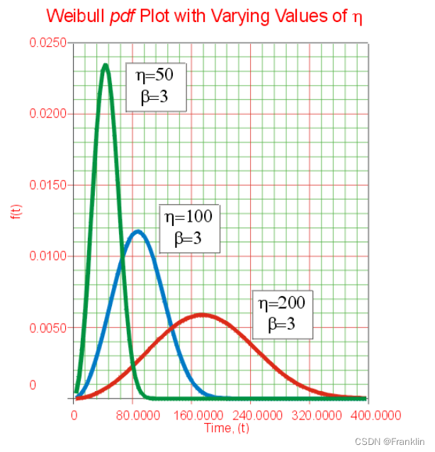
f ( t ; β , η ) = { β η β t β − 1 e − ( t η ) β t , β , η > 0 0 Its He love condition \large\displaystyle f(t;\beta,\eta)=\left\{\begin{matrix} \frac{\beta }{\eta ^{\beta }}t^{\beta -1}e^{-(\frac{t}{\eta })^\beta } & t,\beta,\eta> 0 & \\ 0& Other situations & \end{matrix}\right. f(t;β,η)={ ηββtβ−1e−(ηt)β0t,β,η>0 Its He love condition
- β (shape parameter shape parameter ) Also known as weibull slope Weber slope
- η (scale parameter Scaling parameters )
It looks like this :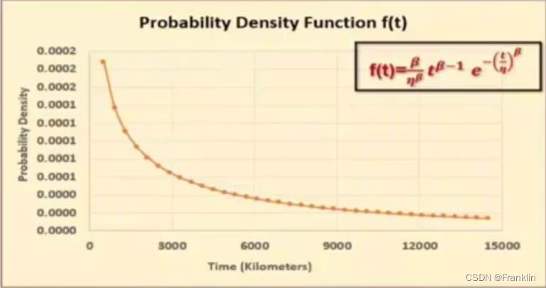
however , Actually, the more detailed definition of Weber distribution is 3 The expression of the parameter .
3.3 Three parameter Weber distribution Weibull Distribution Of PDF(Probability density function)
A continuous random variable X, The three parameter Weber distribution with the following three parameters and density function .
f ( t ; β , η , γ ) = { β η β ( t − γ ) β − 1 e − ( t − γ η ) β t , β , η > 0 0 Its He love condition \large\displaystyle f(t;\beta,\eta,\gamma)=\left\{\begin{matrix} \frac{\beta }{\eta ^{\beta }}(t-\gamma)^{\beta -1}e^{-(\frac{t-\gamma}{\eta })^\beta } & t,\beta,\eta> 0 & \\ 0& Other situations & \end{matrix}\right. f(t;β,η,γ)={ ηββ(t−γ)β−1e−(ηt−γ)β0t,β,η>0 Its He love condition
- β (shape parameter shape parameter ) Also known as weibull slope Weber slope
- η (scale parameter Scaling parameters )
- γ (location parameter Positional arguments , Also known as threshold Threshold parameters )
【 case , so , When γ=0 When , A three parameter distribution becomes a two parameter distribution 】
3.4 Single parameter - standard Weibull Distribution Of PDF

【 Case extract , The Greek alphabet is a little different 】
4 Failure rate function (Hazard Rate or Failure rate Function)
h ( t ) = f ( t ) R ( t ) = β η β t β − 1 e − ( t η ) β e − ( t η ) β = β η β . t β − 1 \large\displaystyle h(t) =\frac{f(t)}{R(t)}=\frac{\frac{\beta }{\eta ^{\beta }}t^{\beta -1}e^{-(\frac{t}{\eta })^\beta }}{ e^{-(\frac{t}{\eta })^{\beta }}}=\frac{\beta}{\eta^\beta}.t^{\beta-1} h(t)=R(t)f(t)=e−(ηt)βηββtβ−1e−(ηt)β=ηββ.tβ−1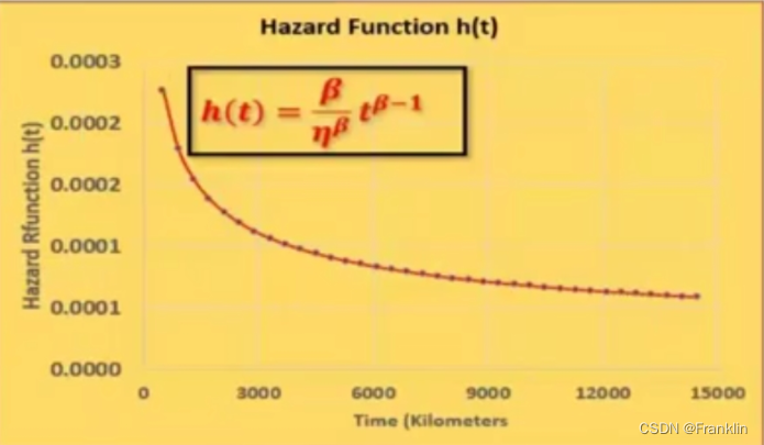
5 Mathematical expectation or life expectancy calculation ( Weibull mean life or MTTF)
【 Three parameter formula 】
E ( X ) = η Γ ( 1 + 1 β ) + μ \large\displaystyle E(X) =\eta \Gamma \left( 1+\frac{1}{\beta } \right)+\mu E(X)=ηΓ(1+β1)+μ
【 Two parameter formula 】
E ( X ) = η Γ ( 1 + 1 β ) \large\displaystyle E(X) =\eta \Gamma \left( 1+\frac{1}{\beta } \right) E(X)=ηΓ(1+β1)
Γ ( x ) \Gamma(x) Γ(x)【 case , Here comes the gamma function , There are more detailed descriptions in the reference list 】
6 Variance formula (Variance)
σ = η 2 [ Γ ( 1 + 2 β ) − Γ 2 ( 1 + 1 β ) ] \large\displaystyle \sigma ={ {\eta }^{2}}\left[ \Gamma \left( 1+\frac{2}{\beta } \right)-{ {\Gamma }^{2}}\left( 1+\frac{1}{\beta } \right) \right] σ=η2[Γ(1+β2)−Γ2(1+β1)]
7 Other related definition formulas
7.1 skewness (skewness)

7.2 kurtosis (kurtosis)

7.3 The median equation , Or call it B50 The formula
【 case , It is used to calculate the maintenance period of a car, for example 、 Or the calculation of intermediate maintenance of other systems 】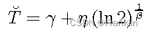
7 Noun reference :
7.0 Cumulative distribution :(Cumulative Density)CDF
Fx(x) = P(X ≤ x) [CDF It is all possible probabilities before accumulating random variables .【 case , Generally use large F(x) describe 】
【 case , A simple example , Throw dice , It's a random event 6 The probability of different results is the same , that , get 1 The probability of a point is 1/6, get 2 The probability of a point is also 1/6, that , get 2 Probability of the following points , Is to obtain 1 The sum of the probabilities of points 2 The sum of the probabilities of points , That is, cumulative probability , It can be expressed as less than or equal to 2 The probability of 1/6 + 1/6 = 2/6 = 1/3】
So there is :
Probability of getting 1 = P(X≤ 1 ) = 1 / 6
Probability of getting 2 = P(X≤ 2 ) = 2 / 6
Probability of getting 3 = P(X≤ 3 ) = 3 / 6
Probability of getting 4 = P(X≤ 4 ) = 4 / 6
Probability of getting 5 = P(X≤ 5 ) = 5 / 6
Probability of getting 6 = P(X≤ 6 ) = 6 / 6 = 1
This is discrete ,
Where X is the probability that takes a value less than or equal to x and that lies in the semi-closed interval (a,b], where a < b.
P(a < X ≤ b) = Fx(b) – Fx(a)
If , Make it continuous , that ,CDF It can be seen as PDF Integral , The following example shows this relationship :
It is known that PDF,
seek CDF,
7.1 Probability density :(Probability Density)PDF
Probability density , General description , You can refer to the reference link at the end of the article . Here is a brief summary .
We understand probability density ,PD, It can be considered as the probability of a random event . then , The value of this probability p(x), It has a corresponding relationship with the random events , We can think of it as a function ,f(x).
x The definition domain of is understood as the definition interval related to probability , The probability of an event occurring at random . The probability of occurrence of events in all intervals is obviously 1.
Simply speaking, probability density has no practical significance , It must have a definite bounded interval . The probability density can be regarded as the ordinate , The interval is regarded as the abscissa , The integral of the probability density over the interval is the area , And this area is the probability of the event occurring in this interval , The sum of all areas is 1
For random variables X Distribution function of F(x), If there is a nonnegative integrable function f(x), So that for any real number x, Yes 
be X Is a continuous random variable , call f(x) by X The probability density function of , Referred to as Probability density .
【 case , Generally use large F(x) describe CDF,f(x) describe PDF】
7.2 Gamma function
Gamma function can be seen everywhere in mathematics .
From Statistics , number theory , Complex analysis in mathematics , To string theory in physics . It seems to be a mathematical glue , Connect different areas .
1738 year , The great Euler , Aspire to extend factorial to non integer range .
Γ ( n ) = ( n − 1 ) ! \large\displaystyle \Gamma \left( n \right)=\left( n-1 \right)! Γ(n)=(n−1)!
【 For this derivation, please refer to the link at the end of the article , All in all , The gamma function can be expressed as the following expression from discrete to continuous 】
Γ ( n ) = ∫ 0 ∞ t n − 1 e − t d t \large\displaystyle \Gamma \left( n \right)=\int _{0}^{\infty }{ { {t}^{n-1}}}{ {e}^{-t}}dt Γ(n)=∫0∞tn−1e−tdt
7.2.1 Properties of gamma function :

7.2.2 Gamma distribution :

7.2.3 Mathematical expectation and variance of gamma distribution 
7.3 Mathematical expectation 【 mean value 】
7.3.1 Definition :
Namely mean value : In probability and Statistics , Mathematical expectation (mathematic expectation [4] )( Or the average , Also called expectation )
Is the probability of each possible result in the test multiplied by the sum of its results , Is one of the most basic mathematical characteristics . It reflects Average value of random variable Size .
expression ,E(x)
7.3.2 The story of origin :
stay 17 century , A gambler challenged Pascal, a famous French mathematician , Gave him a title : A and B gamble , The two of them have an equal chance of winning , The rule of the game is to win three games first , There are five games in total , The winner can get 100 The reward of francs . When the game reaches the fourth inning , A won two games , B won a game , At this time, for some reason, the game was suspended , So how to distribute this 100 Francs are fair ?
With the knowledge of probability theory , It's not hard to know , A is more likely to win , B has little chance of winning .
Because the possibility of a losing the last two games is only (1/2)×(1/2)=1/4, That is to say, the probability of a winning the last two games or any one of the last two games is 1-(1/4)=3/4, Jiayou 75% Expect to get 100 franc ; And B expects to win 100 Franc will have to beat a in both the last two games , The probability of B winning the last two games in a row is (1/2)(1/2)=1/4, That is, B has 25% Expect to get 100 Franc bonus .
so , Although we can't play any more , But based on the above possibilities , The objective expectations for the final victory of Party A and Party B are 75% and 25%, Therefore, a should share the bonus 10075%=75( franc ), B should get the bonus 100×25%=25( franc ). There's something in this story “ expect ” The word , Mathematical expectations come from this .
7.3.3 Continuous mathematical expectation
Let continuous random variable X The probability density function of is f(x), If integral converges absolutely , Then the value of the integral

Is the mathematical expectation of random variables , Write it down as E(X).
7.4 Gaussian distribution
Normal Probability Distribution Formula
P ( x ) = 1 2 π σ 2 e − ( x − μ ) 2 / 2 σ 2 \begin{array}{l}\large P(x)=\frac{1}{\sqrt{2\pi \sigma ^{2}}} e^{-(x-\mu )^{2}/2\sigma ^{2}}\end{array} P(x)=2πσ21e−(x−μ)2/2σ2
μ = Mean
σ = Standard Distribution.
x = Normal random variable.
Literature reference :
Cumulative Distribution Function
Weibull Distribution , ASQ ,Hemant Urdhwareshe
Characteristics of the Weibull Distribution
The New Weibull Handbook
The most beautiful function in the world ——γ function , A pearl on the crown of mathematics
Understanding Probability Distributions
边栏推荐
- 手写MapReduce程序详细操作步骤
- 如何优化PlantUML流程图(时序图)
- C language structure - learning 27
- Jmeter接口测试之常用断言
- Forecast report on industry operation and development strategy of global and Chinese suspension control station industry 2022-2028
- 关于 MySQL 修改密码失败
- Tencent programmer roast: 1kW real estate +1kw stock +300w cash, ready to retire at the age of 35
- websocket服务器实战
- jmeter 性能测试用 csv,这个坑有些扯蛋
- 2022 edition of global and Chinese hexamethylene chloride industry dynamic research and investment prospect forecast report
猜你喜欢

新知识:Monkey 改进版之 App Crawler

Matlab 基础04 - 冒号Colon operator “:”的使用和复杂应用详析

Creating a flutter high performance rich text editor - rendering

Yixin Huachen talks about how to do a good job in customer master data management

在玻璃上构建电路

Ms-hgat: information diffusion prediction based on memory enhanced sequence hypergraph attention network

Kill session? This cross domain authentication solution is really elegant
Weibull Distribution韦布尔分布的深入详述(2)参数和公式意义

jmeter 性能测试用 csv,这个坑有些扯蛋

功能测试如何1个月快速进阶自动化测试?明确这2步就问题不大了
随机推荐
Esp8266wifi development board collects temperature and humidity data and uploads them to the Internet of things platform
2022 edition of global and Chinese on silicon liquid crystal market supply and demand research and prospect Trend Forecast Report
Redis advanced - correspondence between object and code base
[path of system analysts] summary of real problems of system analysts over the years
ROS2之OpenCV基础代码对比foxy~galactic~humble
验证码是自动化的天敌?看看阿里P7大神是怎么解决的
Codemirror 2 - highlight only (no editor) - codemirror 2 - highlight only (no editor)
Low code platform design exploration, how to better empower developers
2022 edition of global and Chinese hexamethylene chloride industry dynamic research and investment prospect forecast report
Article 4: Design of multifunctional intelligent trunk following control system | undergraduate graduation project - [data search skills + reference resource integration]
How to guarantee industrial control safety: system reinforcement
如何优化PlantUML流程图(时序图)
Lambda intermediate operation skip
Lambda intermediate operation limit
Current situation investigation and demand forecast report of global and Chinese phenolic resin market, 2022 Edition
【ROE】(2)ROE协议
Forecast report on market demand and future prospect of cvtf industry of China's continuously variable transmission oil
Lambda quick start
Lambda中间操作sorted
Crawler case 05 - parsing websites using XPath