SOM Network 1: Principles Explained

SOM 介绍

SOM (Self Organizing Maps):自组织映射神经网络,是一种类似于kmeans``的聚类算法,for finding data聚类中心.它可以将The relationship is complex and nonlinearhigh latitude data,Mapping to have simple geometry and interrelationshipslow-latitude space.（Low-latitude maps can reflect the topological structure between high-latitude features）

• 自组织映射(Self-organizing map, SOM)通过学习输入空间中的数据,生成一个低维、离散的映射(Map),To some extent, it can also be regarded as one降维算法.
• SOM是一种无监督的人工神经网络.不同于一般神经网络基于损失函数的反向传递来训练,它运用竞争学习(competitive learning)策略,依靠神经元之间互相竞争逐步优化网络.且使用Neighbor relation function(neighborhood function)to maintain the input space拓扑结构.
• 由于基于无监督学习,这意味着训练阶段不需要人工介入(即不需要样本标签),我们可以在不知道类别的情况下,对数据进行聚类;可以识别针对某问题具有内在关联的特征.
• Data visualization can be achieved;聚类;分类;特征抽取等任务

特点归纳

• 神经网络,竞争学习策略
• 无监督学习,不需要额外标签
• Great for visualization of high-dimensional data,能够维持输入空间的拓扑结构
• 具有很高的泛化能力,It can even recognize input samples it has never encountered before

网络结构

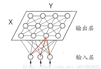
SOMThe network structure has2层：输入层、输出层(Also called the competition layer),.

• 输入层 :包含D个节点,The number of nodes is determined by the dimension of the input features,Same as input feature dimension.
• 输出层：Usually the nodes of the output layer are arranged in layersX行Y列的矩阵形式,输出层有X x Y个节点.

网络的特点

• (1) each node of the output layer,通过Dright side,with all sample pointsDdimensional eigenvectors are connected.,输出层$i,j$ A node vector of locations：
  $$W_{ij}=[w_{ij0},w_{ij0},...w_{ijD}]$$
  换句话说：输出层$i,j$ A node for a location can use oneD维矢量$W_{ij}$来表征`
• (2) 经过训练后,between each node of the output layer,There is a certain correlation according to distance,That is, the closer you are,关联度越高,It can also be expressed as two points that are closer to each other,This is two pointsD维矢量will be closer.
• (3) 训练的目的:学习X x Y个D维权重$W$,All training samples can be used(每个样本D维特征向量)Map to the nodes of the output layer.
  High latitude space(输入)距离近的点,The distance is also closer after mapping to the output layer.For example, two sample points are relatively close to each other$(i,j)$上,或者映射到$(i,j)$和$(i,j+1)$上.

模型训练过程

• 1 准备训练数据datas：N x D N为样本的数量,Dis the dimension of the feature vector for each sample
  通常需要正则化：
  $$datas=\frac{datas-mean(datas)}{std(datas)}$$
• 2.确定参数 $X,Y$$X=Y=\sqrt{5\sqrt{N}}$ , 向上取整
• 3.权重$W$ 初始化: $W$的维度为(X x Y x D)
• 4.迭代训练
  1） Read a sample point $x$ : [D] # D维
  2） 计算样本$x$ respectively with the output layer $X\ast Y$nodes to calculate the distance,找到距离最近的点$(i,j)$作为激活点,set its weight$g$为1
  3） for other nodes in the output layer,Take advantage of it and location$(i,j)$node distance at ,Calculate their weights$g$,与$(i,j)$The closer the location is,则权重越大. Complete the calculation of the output layerX*Y节点权重$g$,特点是以$(i,j)$where the weight is the largest,The farther away it is, the smaller it is
  
• 4） Update the representation vectors of all nodes in the output layer：
  $$W=W+\eta \ast g\ast (x-W)$$
  其中$\eta$是学习率,$x-W$Represents the currently updated output layer node and input samplex的距离,The purpose of updating a node's representation vector is to make the node approximate the input vector$x$

整个SOM映射过程,Equivalent to inputNsamples for cluster mapping,比如输入样本$x1$,$x2$,$x3$ Maps to output nodesa, 样本$x4$,$x5$,$x6$Maps to output nodesb,Then you can use the output nodeato characterize the sample$x1$,$x2$,$x3$;Use output nodesbto characterize the sample$x4$,$x5$,$x6$

5. 经过多轮迭代,Finished characterizing the output node vector$W$的更新,The representation vectors of these nodes can characterize the input samplesx （N x D）.Equivalent to taking the input sample,映射为(XxYxD)的表征向量$W=w_{1,1},w_{1,2},,,w_{x,y}$

权重初始化 W：[X,Y,D]

Weight initialization mainly includes3种方法：

• 1 随机初始化,然后标准化 $W=\frac{W}{||W||}$
• 2 Picked randomly from the training data$X\ast Y$个,来初始化权重
• 3 对训练数据进行PCA,Take the two eigenvectors with the largest eigenvaluesM: D x 2 Mapping as a basis vector.

距离计算方式

采用欧式距离计算 ,公式如下：
$$dis=||x-y||$$

Calculate the weights of the output nodesg

Suppose the activation point coordinates are $(c_X,c_y)$ ,其他位置 $i,j$处的权重gThere are two main methods of calculation：

• 高斯法

$$g(i,j)=e^{-\frac{(c_x-i{)}^2}{2{\sigma }^2}}{e}^{-\frac{(c_y-j{)}^2}{2{\sigma }^2}}$$
可以看出到$（i,j）$is the activation point$(c_X,c_y)$,计算得到的g=1.The weights exhibit a Gaussian distribution.Among them the Gaussian method$\sigma$The value also changes with the number of iteration steps,更新方式跟学习率方式一样,参见后面学习率的更新

• Hard threshold method
  
  这种方法比较直接,以$(c_X,c_y)$within a certain range of the centerg为1,其他为0,;Generally, the Gaussian method is selected

学习率更新

$$\eta =\frac{{\eta }_0}{1+\frac{t}{ma{x}_{step}/2}}$$

其中$t$Indicates the current iterationstep,$ma{x}_{step}$The total number of iterations for network training,学习率$\eta$随着迭代次数的增加,会越来越小.