Random forest project combat - temperature prediction

The three tasks of the actual combat project：

1.Basic modeling is done using the random forest algorithm：包括数据预处理,特征展示,Complete modeling and perform visual display analysis.

2.Analyze the impact of the data sample size and the number of features on the results,On the premise of ensuring that the algorithm is consistent,Increase the number of samples,Observe that the results change,Re-engineer the feature,After introducing new features,Observe the trend of the results.

3.Adjust the parameters of the random forest algorithm,找到最合适的参数,Master two methods of parameter tuning in machine learning,Find the optimal parameters of the model.

任务1：

import pandas as pd
data =pd.read_csv()
data.head()
import datetime
year = data['year']
month  =data['month']
day =data['day']
dates = [(str(year)+'-'+str(month)+'-'+str(day)) for year,month,day in  zip(year,month,day)]
dates=[datetime.datetime.strptime(date,'%Y-%m-%d') for date in dates]
dates[:5]

Rescale the time series,Do feature drawing.

##进行绘图
import matplotlib.pyplot as plt
%matplotlib inline
plt.style.use('fivethirtyeight')##风格设置
# 设置布局
fig, ((ax1, ax2), (ax3, ax4)) = plt.subplots(nrows=2, ncols=2, figsize = (10,10))
fig.autofmt_xdate(rotation = 45)

# 标签值
ax1.plot(dates, data['actual'])
ax1.set_xlabel(''); ax1.set_ylabel('Temperature'); ax1.set_title('Max Temp')

# 昨天
ax2.plot(dates, data['temp_1'])
ax2.set_xlabel(''); ax2.set_ylabel('Temperature'); ax2.set_title('Previous Max Temp')

# 前天
ax3.plot(dates, data['temp_2'])
ax3.set_xlabel('Date'); ax3.set_ylabel('Temperature'); ax3.set_title('Two Days Prior Max Temp')

# 我的逗逼朋友
ax4.plot(dates, data['friend'])
ax4.set_xlabel('Date'); ax4.set_ylabel('Temperature'); ax4.set_title('Friend Estimate')

plt.tight_layout(pad=2)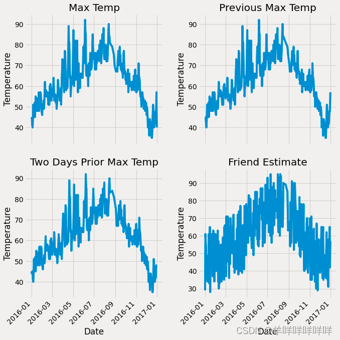

从中可以看出4The basic influence of a feature on the trend.

import numpy as np
y = np.array(data['actual'])
x = data.drop(['actual'],axis=1)
x_list =list(x.columns)
x = np.array(x)
##数据分类
from sklearn.model_selection import train_test_split
x_train,x_test,y_train,y_test =train_test_split(x,y,test_size=0.25,random_state=42)
##建立随机森林模型
from sklearn.ensemble import RandomForestRegressor
rfr = RandomForestRegressor(n_estimators=1000,random_state=42)
rfr.fit(x_train,y_train)
y_pred = rfr.predict(x_test)
from sklearn.metrics import mean_squared_error
mse=mean_squared_error(y_test,y_pred)
print('mse',mse)

 Here, the splitting of the test set and the training set and the establishment of the random forest model are carried out.The result and the real value calculation amount are predicted by the established modelmse的值.

The visualization of the decision tree was followed

from sklearn.tree import export_graphviz
import pydot
tree = rfr.estimators_[5]
export_graphviz(tree,out_file='tree.dot',
               feature_names=x_list,
               rounded=True,precision=1)
(graph,) = pydot.graph_from_dot_file('tree.dot')
graph.write_png('tree.png')

Because the branches are too complex and numerous,So do pre-pruning.

##Do pre-pruning
rfr_small = RandomForestRegressor(n_estimators=10,max_depth=3,random_state=42)
rfr_small.fit(x_train,y_train)
tree_small = rfr_small.estimators_[5]
export_graphviz(tree_small,out_file='small_tree.dot',
               feature_names=x_list,
               rounded=True,precision=1)
(graph,) = pydot.graph_from_dot_file('small_tree.dot')
graph.write_png('small_tree.png')

2.Select key features,The results for the full feature and the focused feature are then compared

这里使用了randomforestregressor.feature_importance_Important values ​​can be output.

##通过randomforestregressor的feature_importance_显示特征重要性
importance = list(rfr.feature_importances_)
feature_importances =[(feature_name,importance) for feature_name,importance in zip(x_list,importance)]
feature_importances =sorted(feature_importances,key =lambda x:x[1],reverse =True)##key To use that column of data as the arrangement object
feature_importances
##Calculate with these two features as the only two features
rfr = RandomForestRegressor(n_estimators=100,random_state=42)
new_x = np.array(data.iloc[:,4:5])
new_x_train,new_x_test,new_y_train,new_y_test =train_test_split(new_x,y,test_size=.25,random_state=42)
rfr.fit(new_x_train,new_y_train)
y_pred = rfr.predict(new_x_test)
print('mse',mean_squared_error(new_y_test,y_pred))

相比之下,mse值上升,Description is not good,Other features have important effects as well.

任务二：Analysis of the impact of data and features on results.

The expansion package that reads the data is tested here.The operation is the same as above

import pandas as pd
data =pd.read_csv()
data.head()
##绘图观察数据
# Convert to standard format
import datetime

# Get various date data
years = data['year']
months = data['month']
days = data['day']

# 格式转换
dates = [str(int(year)) + '-' + str(int(month)) + '-' + str(int(day)) for year, month, day in zip(years, months, days)]
dates = [datetime.datetime.strptime(date, '%Y-%m-%d') for date in dates]

# 绘图
import matplotlib.pyplot as plt

%matplotlib inline

# 风格设置
plt.style.use('fivethirtyeight')
# Set up the plotting layout
fig, ((ax1, ax2), (ax3, ax4)) = plt.subplots(nrows=2, ncols=2, figsize = (15,10))
fig.autofmt_xdate(rotation = 45)

# Actual max temperature measurement
ax1.plot(dates, data['actual'])
ax1.set_xlabel(''); ax1.set_ylabel('Temperature (F)'); ax1.set_title('Max Temp')

# Temperature from 1 day ago
ax2.plot(dates, data['temp_1'])
ax2.set_xlabel(''); ax2.set_ylabel('Temperature (F)'); ax2.set_title('Prior Max Temp')

# Temperature from 2 days ago
ax3.plot(dates, data['temp_2'])
ax3.set_xlabel('Date'); ax3.set_ylabel('Temperature (F)'); ax3.set_title('Two Days Prior Max Temp')

# Friend Estimate
ax4.plot(dates, data['friend'])
ax4.set_xlabel('Date'); ax4.set_ylabel('Temperature (F)'); ax4.set_title('Friend Estimate')

plt.tight_layout(pad=2)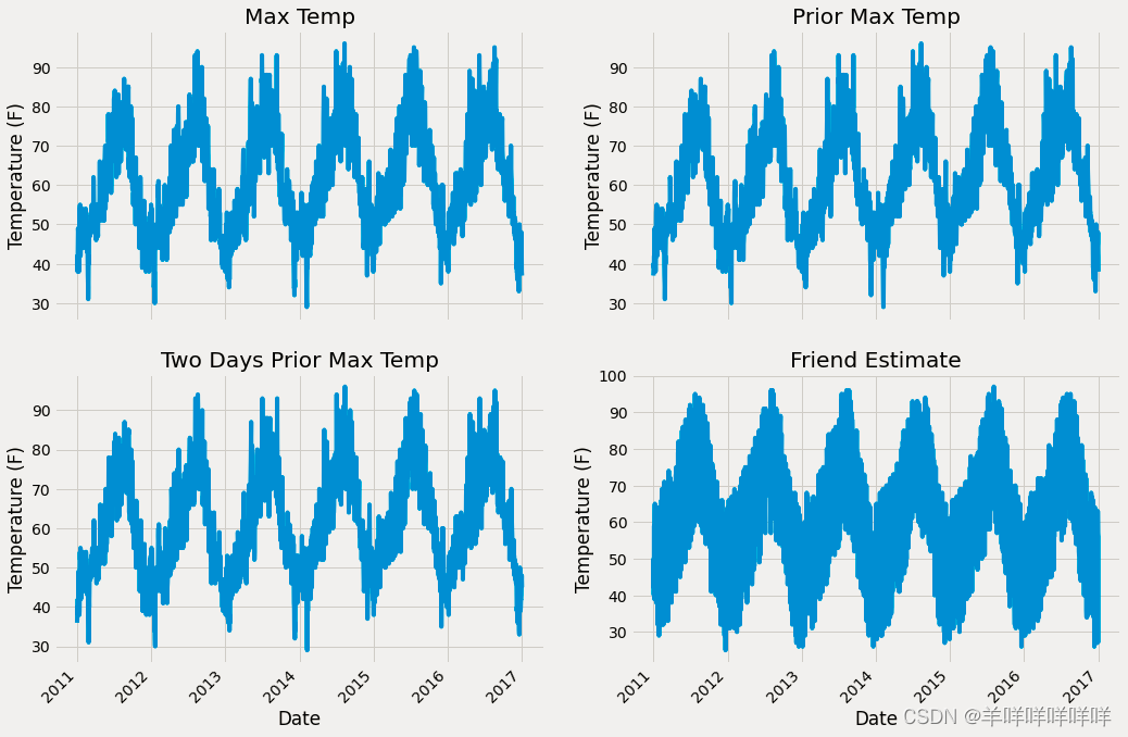

 Because of more features,Combine and process the extra features.

seasons=[]
for month in data['month']:
    if month in[1,2,12]:
        seasons.append('winter')
    elif month in [3,4,5]:
        seasons.append('spring')
    elif month in [6,7,8]:
        seasons.append('summer')
    else:
        seasons.append('auntumn')
reduced_x = data[['temp_1','prcp_1','average','actual']]
reduced_x['seasons']=seasons
# 导入seaborn工具包
import seaborn as sns
sns.set(style="ticks", color_codes=True);

# Choose your favorite color template
palette = sns.xkcd_palette(['dark blue', 'dark green', 'gold', 'orange'])

# 绘制pairplot
sns.pairplot(reduced_x, hue = 'seasons', diag_kind = 'kde', palette= palette, plot_kws=dict(alpha = 0.7),
                   diag_kws=dict(shade=True));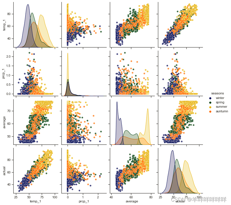 

 A correlation graph of temperature changes over four months is drawn.

Change the amount of data first,The impact of the amount of test data on the model performance.

data = pd.get_dummies(data)
new_y = np.array(data['actual'])
new_x = data.drop(['actual'],axis=1)
new_x_list =list(new_x.columns)
new_x = np.array(new_x)
from sklearn.model_selection import train_test_split
new_x_train,new_x_test,new_y_train,new_y_test =train_test_split(new_x,new_y,test_size=0.25,random_state=42)
old_y = np.array(data['actual'])
old_x = data.drop(['actual'],axis=1)
old_x_list =list(old_x.columns)
old_x = np.array(old_x)
from sklearn.model_selection import train_test_split
old_x_train,old_x_test,old_y_train,old_y_test =train_test_split(x,y,test_size=0.25,random_state=42)
def model_train_predict(x_train,y_train,x_test,y_test):
    rfr = RandomForestRegressor(n_estimators=100,random_state=42)
    rfr.fit(x_train,y_train)
    y_pred = rfr.predict(x_test)
    errors= abs(y_pred-y_test)
    print('平均误差',round(np.mean(errors),2))
    accuracy = 100-np.mean(errors)
    print('平均正确率',accuracy)
model_train_predict(old_x_train,old_y_train,old_x_test,old_y_test)
model_train_predict(ori_new_x_train,new_y_train,ori_new_x_test,new_y_test)

从结果可以发现,当数据量增加,误差减少.

Then change the number of features,Determine its effect on the effect.

rfr = RandomForestRegressor(n_estimators=100,random_state=42)
rfr.fit(new_x_train,new_y_train)
y_pred = rfr.predict(new_x_test)
errors= abs(y_pred-new_y_test)
print('平均误差',round(np.mean(errors),2))
accuracy = 100-np.mean(errors)
print('平均正确率',accuracy)
importances = list(rfr.feature_importances_)
feature_importances  =[(feature,importance) for feature,importance in zip(new_x_list,importances)]
feature_importances = sorted(feature_importances,key =lambda x:x[1],reverse =True)
# 对特征进行排序
x_values =list(range(len(importances)))
sorted_importances = [importance[1] for importance in feature_importances]
sorted_features = [importance[0] for importance in feature_importances]

# cumulative importance
cumulative_importances = np.cumsum(sorted_importances)

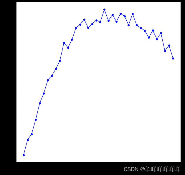
# 绘制折线图
plt.plot(x_values, cumulative_importances, 'g-')

# Draw a red dotted line,0.95那
plt.hlines(y = 0.95, xmin=0, xmax=len(sorted_importances), color = 'r', linestyles = 'dashed')

# X轴
plt.xticks(x_values, sorted_features, rotation = 'vertical')

# Yaxis and name
plt.xlabel('Variable'); plt.ylabel('Cumulative Importance'); plt.title('Cumulative Importances');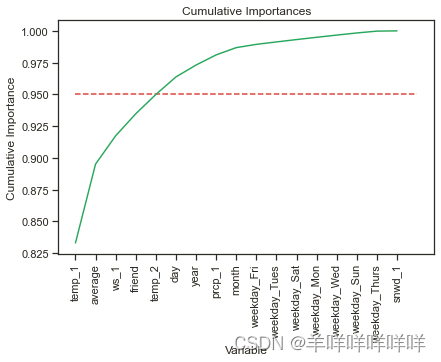

 According to principal component analysis,Overall importance is greater than 95%Basically it can be summed up as this5A feature can cover all importance.

important_feature_names =[feature[0] for feature in feature_importances[0:5]]
important_feature_indices =[new_x_list.index(feature) for feature in important_feature_names]
important_x_train = new_x_train[:,important_feature_indices]
important_x_test = new_x_test[:,important_feature_indices]
model_train_predict(important_x_train,new_y_train,important_x_test,new_y_test)
##Runtime improvement
import time 
all_features_time=[]
for _ in range(10):
    start_time = time.time()
    rfr.fit(new_x_train,new_y_train)
    y_pred = rfr.predict(new_x_test)
    end_time =time.time()
    all_features_time.append((end_time-start_time))
all_features_times=np.mean(all_features_time)
all_features_time=[]
for _ in range(10):
    start_time = time.time()
    rfr.fit(important_x_train,new_y_train)
    y_pred = rfr.predict(important_x_test)
    end_time =time.time()
    all_features_time.append((end_time-start_time))
reduced_features_times=np.mean(all_features_time)
all_accuracy =100*(1-np.mean(abs(all_y_pred-new_y_test)/new_y_test))
reduced_accuracy =100*(1-np.mean(abs(reduced_y_pred-new_y_test)/new_y_test))
comparison = pd.DataFrame({'features': ['all (17)', 'reduced (5)'], 
                           'run_time': [all_features_times, reduced_features_times],
                           'accuracy': [all_accuracy, reduced_accuracy]})

comparison[['features', 'accuracy', 'run_time']]

Here, the optimization of the running time is compared with the improvement of the accuracy rate,It is found that when the amount of data is large and there are many features,The better the model is built.

任务三：调参：这里使用RandomizeSearchCV与GridSearchCVThere are two ways to adjust parameters for parameter selection.

from sklearn.model_selection import RandomizedSearchCV
n_estimators =[int(x) for x in np.linspace(start=200,stop=2000,num=10)]
max_features=['auto','sqrt']
max_depth = [int(x) for x in np.linspace(10,20,num=2)]
max_depth.append(None)
min_samples_split=[2,5,10]
min_samples_leaf=[1,2,4]
bootstrap = [True,False]
random_grid = {'n_estimators': n_estimators,
               'max_features': max_features,
               'max_depth': max_depth,
               'min_samples_split': min_samples_split,
               'min_samples_leaf': min_samples_leaf,
               'bootstrap': bootstrap}
rf = RandomForestRegressor()

rf_random = RandomizedSearchCV(estimator=rf, param_distributions=random_grid,
                              n_iter = 100, scoring='neg_mean_absolute_error', 
                              cv = 3, verbose=2, random_state=42, n_jobs=-1)

# Perform a seek operation
rf_random.fit(new_x_train, new_y_train)
from sklearn.model_selection import GridSearchCV

# 网络搜索
param_grid = {
    'bootstrap': [True],
    'max_depth': [8,10,12],
    'max_features': ['auto'],
    'min_samples_leaf': [2,3, 4, 5,6],
    'min_samples_split': [3, 5, 7],
    'n_estimators': [800, 900, 1000, 1200]
}

# Select the base algorithm model
rf = RandomForestRegressor()

# 网络搜索
grid_search = GridSearchCV(estimator = rf, param_grid = param_grid, 
                           scoring = 'neg_mean_absolute_error', cv = 3, 
                           n_jobs = -1, verbose = 2)
grid_search.fit(train_features, train_labels)

Finally, it is found that the general direction can be determined by random search,Refine your search using gridded search