Feature dimensionality reduction study notes (pca and lda) (1)

There are two mainstream dimensionality reduction methods：Projection and Manifold Learning,Projection refers to projecting high-dimensional data onto a low-dimensional plane,But it can cause subspace twiddles.Whereas, manifold learning relies on manifold design,Manifold design mainly considers real-world high-dimensional datasets to be close to low-dimensional fluids.

主成分分析（PCA）：It is projected by identifying hyperplanes close to the data,Essentially by comparing the original datasets,The variance to the new plane is minimal,is the first principal component,When the covariance of the second principal component and the first component is 0,说明不相关,is the second principal component,以此类推.

使用python计算pca：

import  numpy as np
np.random.seed(4)
m = 60
w1, w2 = 0.1, 0.3
noise = 0.1

angles = np.random.rand(m) * 3 * np.pi / 2 - 0.5
X = np.empty((m, 3))
X[:, 0] = np.cos(angles) + np.sin(angles)/2 + noise * np.random.randn(m) / 2
X[:, 1] = np.sin(angles) * 0.7 + noise * np.random.randn(m) / 2
X[:, 2] = X[:, 0] * w1 + X[:, 1] * w2 + noise * np.random.randn(m)
X_centered = X-X.mean(axis=0)
U,S,Vt =np.linalg.svd(X_centered)
c1 = Vt.T[:,0]
c2 = Vt.T[:,1]
w2 =Vt.T[:,:2]
X2D = X_centered.dot(w2)
X2D

这里使用了svd方法（奇异值分解）,Its role is to rotate the coordinate axis,Rotate after stretching,The purpose of calculating the mean is in the process of calculating the principal components,It is necessary to obtain the mean of each class of principal components,Then the mean point distance of each class of principal components is maximized,The difference between the sample points of each type is the smallest.

使用sklearn中的decomposition的pca方法进行模拟

from sklearn.decomposition import PCA
pca =PCA(n_components=2)
X_2D =pca.fit_transform(X)
pca.components_.T[:,0]##Unit vector of the first principal component

在主成分分析中,有一类方法,Cumulatively find the sum of the principal components,When the total principal components are greater than 95%时,Take these principal components as the total score for calculation.

pca.explained_variance_ratio_##Explained variance ratio,Indicate the proportion of variance of the first two principal components

这里使用pca的函数explained_variance_ratio可解释方差,The essence is the importance of features.

from sklearn.datasets import fetch_openml
mnist = fetch_openml('mnist_784', version=1, as_frame=False)
mnist.target = mnist.target.astype(np.uint8)
from sklearn.model_selection import train_test_split
X = mnist["data"]
y = mnist["target"]
X_train, X_test, y_train, y_test = train_test_split(X, y)
pca = PCA()
pca.fit_transform(X_train)
cumsum = np.cumsum(pca.explained_variance_ratio_)##Sum the data row by row
d = np.argmax(cumsum>0.95)+1

也可以通过pcaset the hyperparameters

pca = PCA(n_components=0.95)
X_reduced = pca.fit_transform(X_train)

也可以在pca中设置参数,对数据进行压缩

##使用pca进行压缩
pca = PCA(n_components=154)
x_reduced = pca.fit_transform(X_train)
x_reversed = pca.inverse_transform(x_reduced)

pca.inverse_transformCompression features can be restored.

随机pca：Quick find befored个主成分的近似值.pca中的svd_solver='randomized'

rnd_pca = PCA(n_components=154,svd_solver = 'randomized')
x_reduced = rnd_pca.fit_transform(X_train)
rnd_pca.explained_variance_ratio_.sum()

增量pca：Send small batches of data into memory for dimensionality reduction,Enter a small amount of data when done,增加运行速度,Also saves memory space.这里使用了sklearn.decomposition.incrementalPCA

from sklearn.decomposition import IncrementalPCA
IPCA  =IncrementalPCA(n_components=154)
n_batches=100
for x_batch in np.array_split(X_train,n_batches):
    IPCA.partial_fit(x_batch)
x_reduced  =IPCA.transform(X_train)

 也可以使用np.menmap类进行操作.

filename = "my_mnist.data"
m, n = X_train.shape

X_mm = np.memmap(filename, dtype='float32', mode='write', shape=(m, n))
X_mm[:] = X_train
X_mm = np.memmap(filename, dtype="float32", mode="readonly", shape=(m, n))

batch_size = m // n_batches
inc_pca = IncrementalPCA(n_components=154, batch_size=batch_size)
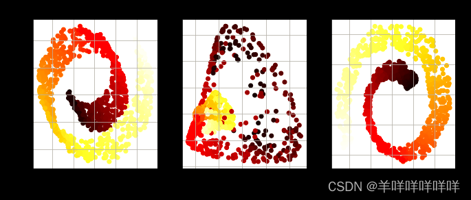
inc_pca.fit(X_mm)

内核pca：Can solve nonlinear complex projections,Grid search can be usedGridSearchCV进行筛选.

from sklearn.decomposition import KernelPCA
from sklearn.datasets import make_swiss_roll
X, t = make_swiss_roll(n_samples=1000, noise=0.2, random_state=42)
rbf_pca = KernelPCA(n_components=2,kernel='rbf',gamma=0.04)
x_reduced = rbf_pca.fit_transform(X)
from sklearn.decomposition import KernelPCA
import matplotlib.pyplot as plt

lin_pca = KernelPCA(n_components = 2, kernel="linear", fit_inverse_transform=True)
rbf_pca = KernelPCA(n_components = 2, kernel="rbf", gamma=0.0433, fit_inverse_transform=True)
sig_pca = KernelPCA(n_components = 2, kernel="sigmoid", gamma=0.001, coef0=1, fit_inverse_transform=True)

y = t > 6.9

plt.figure(figsize=(11, 4))
for subplot, pca, title in ((131, lin_pca, "Linear kernel"), (132, rbf_pca, "RBF kernel, $\gamma=0.04$"), (133, sig_pca, "Sigmoid kernel, $\gamma=10^{-3}, r=1$")):
    X_reduced = pca.fit_transform(X)
    if subplot == 132:
        X_reduced_rbf = X_reduced
    
    plt.subplot(subplot)
    #plt.plot(X_reduced[y, 0], X_reduced[y, 1], "gs")
    #plt.plot(X_reduced[~y, 0], X_reduced[~y, 1], "y^")
    plt.title(title, fontsize=14)
    plt.scatter(X_reduced[:, 0], X_reduced[:, 1], c=t, cmap=plt.cm.hot)
    plt.xlabel("$z_1$", fontsize=18)
    if subplot == 131:
        plt.ylabel("$z_2$", fontsize=18, rotation=0)
    plt.grid(True)


plt.show()

from sklearn.model_selection import GridSearchCV
from sklearn.linear_model import LogisticRegression
from sklearn.pipeline import Pipeline

clf = Pipeline([
        ("kpca", KernelPCA(n_components=2)),
        ("log_reg", LogisticRegression(solver="lbfgs"))
    ])

param_grid = [{
        "kpca__gamma": np.linspace(0.03, 0.05, 10),
        "kpca__kernel": ["rbf", "sigmoid"]
    }]

grid_search = GridSearchCV(clf, param_grid, cv=3)
grid_search.fit(X, y)
print(grid_search.best_params_)
rbf_pca = KernelPCA(n_components=2,kernel='rbf',gamma=0.0433,fit_inverse_transform=True)
x_reduced = rbf_pca.fit_transform(X)
X_preimage =rbf_pca.inverse_transform(X_reduced)
from sklearn.metrics import mean_squared_error
mean_squared_error(X,X_preimage)

 习题：使用MNISTdataset to train a random forest classifier,Test its time and performance,Then after dimensionality reduction,Judge its time and performance,进行比较.

from sklearn.datasets import fetch_openml

mnist = fetch_openml('mnist_784', version=1, as_frame=False)
mnist.target = mnist.target.astype(np.uint8)
X = mnist['data']
Y = mnist['target']
from sklearn.model_selection import train_test_split
x_train,x_test,y_train,y_test =train_test_split(X,Y,test_size=10000)
from sklearn.ensemble import RandomForestClassifier
import time
rfc = RandomForestClassifier()
start_time =time.time()
rfc.fit(x_train,y_train)
end_time = time.time()
print(end_time-start_time)
from sklearn.decomposition import PCA
PCA = PCA(n_components=0.95)
x_reduced_train = PCA.fit_transform(x_train)
rfc_pca = RandomForestClassifier()
start_time =time.time()
rfc_pca.fit(x_reduced_train,y_train)
end_time = time.time()
print(end_time-start_time)
from sklearn.metrics import mean_squared_error
from sklearn.metrics import accuracy_score
def model_descirbe(model,x_test):
    y_pred = model.predict(x_test)
    print('mse',mean_squared_error(y_pred,y_test))
    print('accuracy',accuracy_score(y_pred,y_test))
model_descirbe(rfc)
x_reduced_test = PCA.transform(x_test)
model_descirbe(rfc_pca,x_reduced_test)

结果发现：Length of training time after dimensionality reduction,And the mean square error and correct rate are lower than those without dimension reduction