Time series similarity measurement method
Euclidean distance is commonly used to measure the similarity of time series ED(Euclidean distance) And dynamic time warping DTW(Dynamic Time Warping). The whole is divided into two categories : Lock step measurement (lock-step measures) And elasticity measures (elastic measures) . Lock step measurement is the measurement of time series “ one-on-one ” than a ; Elasticity measures allow time series to be measured “ One to many ” Comparison .
Euclidean distance is a lock step measure .

In time series , We usually need to compare the audio differences between the two ends . The length of the two pieces of audio is mostly unequal . In the field of speech processing, different people speak at different speeds . Even if the same person makes the same sound at different times , Nor can it have exactly the same length of time . And everyone's pronunciation speed of different phonemes of the same word is also different , Some people will put "A" This sound drags a little longer , perhaps "i" A little short . In this complex situation , It is impossible to obtain the effective similarity between two time series by using the traditional Euclidean distance ( Distance ).
Here's the picture , Solid line waveform a The point will correspond to the waveform of the dotted line b’ spot , In this way, the traditional calculation of similarity by comparing distances is obviously unreliable . Because obviously , Solid line a The dot corresponds to the dotted line b Point is right .
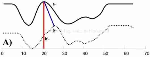
Consider sequences of varying lengths , Or when the time steps are not aligned , Especially at the peak , Euclidean distance is the distance between two time series that cannot be calculated effectively .DTW The algorithm linearly enlarges one of the sequences 、 Do something about “ Distortion ” operation ,. There can be one to many mapping The situation of , In the process of time series exploration, the effect is better . It is suitable for complex time series , It belongs to elasticity measurement

dtw Algorithm is introduced
Suppose we have two time series Q and C, Their lengths are n and m:( Actual time series matching application , A sequence is the reference template , A sequence is the test template )
Q = q1, q2,…,qi,…, qn ;
C = c1, c2,…, cj,…, cm ;
To align the two sequences , We need to construct a n x m Matrix grid of , Matrix elements (i, j) Express qi and cj The distance between two points d(qi, cj)( That's sequence Q Every point and C The similarity between each point of , The smaller the distance, the higher the similarity . No matter the order ), European distance is generally used ,d(qi, cj)= (qi-cj)2( It can also be understood as distortion ). Every matrix element (i, j) Indication point qi and cj Alignment of .DP The algorithm can be reduced to finding a path through several grid points in this grid , The grid point through which the path passes is the alignment point of the two sequences .
So how do we find this path ? Which path is the best ? That's the question just now , How about warping Is the best .
First , This path is not optional , The following constraints need to be met :
1) The boundary conditions :w1=(1, 1) and wK=(m, n). The pronunciation speed of any kind of voice can change , But the order of its parts cannot be changed , Therefore, the selected path must start from the lower left corner , End in the upper right corner .
2) Continuity : If wk-1= (a’, b’), So for the next point of the path wk=(a, b) Need to meet (a-a’) <=1 and (b-b’) <=1. That is, it is impossible to cross a point to match , It can only be aligned with its adjacent points . This ensures Q and C Every coordinate in the is in W It appears that .
3) monotonicity : If wk-1= (a’, b’), So for the next point of the path wk=(a, b) Need to meet 0<=(a-a’) and 0<= (b-b’). This limits W The above points must be monotonous over time . To ensure that B The dashed lines in the do not intersect .
Combine continuity and monotonicity constraints , There are only three directions for each grid point . For example, if the path has passed the grid point (i, j), Then the next passing grid can only be one of the following three cases :(i+1, j),(i, j+1) perhaps (i+1, j+1).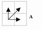
The path satisfying the above constraints can have exponents , The best path is the path that minimizes the accumulation distance along the path . This path can be dynamically planned (dynamic programming) The algorithm gets . Visual examples of specific search or solution processes can be referred to :http://www.cnblogs.com/tornadomeet/archive/2012/03/23/2413363.html
Ordinary dtw Method introduction and use
First step :dtw Package installation , With Anaconda For example
Open... From the start menu Anaconda prompt Management tools
Input dwt set up script
pip install dtw
The second step :dtw Package import
from dtw import dtw
The third step :dtw Function USES
First , You need to define the distance function , among ,x Is the reference sequence data ,y For test sequence data
distance=lambda x,y :np.abs(x-y)
Next , call dtw Method
d,cost_matrix,acc_cost_matrix,path=dtw(x,y,distance)
dtw Function input parameter description
x: Reference sequence data
y: Test sequence data
distance: distance function
dtw Function output parameter description
d: Cumulative distance
cost_matrix: The distance between two sequences
acc_cost_matrix:dp matrix
path: Best path , Contains two arrays ,path[0] Reference sequence subscript value ,path[1] Test sequence subscript value
Print out the trace line
plt.imshow(cost_matrix.T,origin='lower',cmap='gray')
plt.plot(path[0],path[1]) plt.show()
dtw-python Package installation and reference
dtw There are too many restrictions on the use of Libraries , inflexible , And the drawing is not convenient , It mainly reflects the large amount of computation 、 The beginning and end must match 、 The number of correspondences between sequences cannot be limited .dtw-python Bag is R In language dtw Realized python edition , Basic API Is the corresponding , Its advantage is that it can customize the matching pattern of points , constraint condition , And sliding windows . At the same time, it provides convenient drawing and fast calculation (C The kernel of language ), Official documents click here .
dtw-python Package installation script
pip install dtw-python
dtw-python Package reference
from dtw import dtw,dtwPlot,stepPattern,warp,warpArea,window # Direct... Is not recommended from dtw import * The way , To avoid conflict
Because in dtw In the process of package selection , Install the first dtw package , After installing dtw-python package , stay dtw-python During the reference process , appear dtw Package reference failure , It is suggested to retain one of the two . You can use the package uninstall script to dtw Uninstall the package , And in Anaconda Installation directory \Anaconda3\Lib Remove from the directory With ~ Folder named at the beginning
pip uninstall dtw
dtw Parameter description of function
ds=dtw(x, y=None, dist_method='euclidean', step_pattern='symmetric2', window_type=None, window_args={}, keep_internals=False, distance_only=False, open_end=False, open_begin=False)Input parameter description :
dist_method Define the distance method you use , The default is ’euclidean’, Euclidean distance .
keep_internals=True Save internal information, including distance matrix and so on , Generally, we set it to True.
step_pattern Defines the matching pattern between points , There are several kinds. , See the official website for details .
window_type Represents a global conditional constraint , There are also several modes , Check the official website ."none", "itakura", "sakoechiba", "slantedband", among sakoechiba The way needs to be in window_args Parameters window_size Parameters , The way is as follows :window_args= {"window_size": 1}
distance_only If set to True, Will speed up the calculation , Only calculate the distance , Ignore matching functions .
open_end and open_begin Set to True Represents an unrestricted match , That is, a complete partial match , The default is global matching , Is to strictly correspond to the head and tail .
Output parameter description :
ds.distance: Cumulative distance
ds.index1: Reference sequence subscript value
ds.index2: Test sequence subscript value
dtw Print the output result
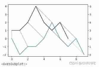
ds.plot(type="twoway",offset=-2)
Generally speaking, there are twoway and threeway Two modes , Here is a detailed explanation ,offset=-2 It can be understood as the degree of separation between two wires , In order to make it easy to see, you can set it larger . On the left side of the picture is twoway Output result of mode , The right side is threeway Output result of mode .

dtw Function usage considerations
1. Empty and invalid values cannot appear in the data , When replacing missing data with the previous record , Missing data in the same period cannot be too much , Otherwise, it will cause large deviation of change trend matching results
2. The maximum and minimum values may not match correctly
dtw Using examples
background : The pollutant concentrations of two sections on the same river show certain similarity in change trend . But due to the uncertainty of river velocity , The time intervals of the peaks and troughs of the concentration in the upstream section are different on the downstream section , Can pass dtw Method to realize the time period of similar change trend between two sections , And the relationship between the changes of pollutant concentration between upstream and downstream sections
First step : add to python Package reference
import numpy as np
import pandas as pd import matplotlib.pylab as plt import math import datetime import time # Used to convert time seconds into time  from dtw import dtw,dtwPlot,stepPattern,warp,warpArea,window # Direct... Is not recommended  from dtw import *  The way , To avoid conflict  import sys import pymssql import xlwt from pandas._libs.tslibs.timestamps import Timestamp
The second step : adopt csv Read the concentration monitoring values of pollutants in two sections in this way
beginTime='2019/1/2 12:00'
endTime='2019/2/18 12:00'

# from csv Extract data from file
df=pd.read_csv('wq3.csv',encoding='utf-8', index_col='datatime') # from csv Read time series data from file ,index_col Columns are defined as index objects
df.index=pd.to_datetime(df.index) df_xy_org=df['qingzhoucun'][beginTime:endTime] # Specify the downstream monitoring data column in the time series  df_sy_org=df['liangtiancun'] # Specify the upstream monitoring data column in the time series  # The missing number needs to be excluded in the specific calculation , Especially the lack of number for a long time , Will affect the final matching result . The method of using the last monitoring data is not appropriate  for i in range(0,len(df_xy_org)): if not df_xy_org[i] or math.isnan(df_xy_org[i]): # Judge whether the value is empty  df_xy_org[i] = df_xy_org[i-1] for i in range(0,len(df_sy_org)): if not df_sy_org[i] or math.isnan(df_sy_org[i]): # Judge whether the value is empty  df_sy_org[i] = df_sy_org[i-1]
The third step : In order to find peaks and troughs more effectively , First order differential treatment of pollutant concentration
# Compare the data to do first-order difference processing
df_xytime=np.empty(len(df_xy_org)-1,dtype=datetime.datetime)
df_xyvalue=np.empty(len(df_xy_org)-1) for i in range(1,len(df_xy_org)-1): df_xytime[i-1]=df_xy_org.index[i].to_pydatetime() df_xyvalue[i-1]=(float(df_xy_org.values[i])-float(df_xy_org.values[i-1])) df_xy=pd.Series(df_xyvalue,index=df_xytime) df_sytime=np.empty(len(df_sy_org)-1,dtype=datetime.datetime) df_syvalue=np.empty(len(df_sy_org)-1) for i in range(1,len(df_sy_org)-1): df_sytime[i-1]=df_sy_org.index[i].to_pydatetime() df_syvalue[i-1]=(float(df_sy_org.values[i])-float(df_sy_org.values[i-1])) df_sy=pd.Series(df_syvalue,index=df_sytime)
Step four : Define the distance function
# Define the distance calculation method
dist=lambda x,y:np.abs(np.power(100,x)-np.power(100,y))
Step five : The downstream section monitoring data is used as the reference sequence , Select... From the monitoring data of upstream section 【 The length of the reference sequence is plus or minus 2 The length of 】 Sequence , Cyclic verification of the most similar time series
#dwt Calculation , comparison dist In the generated results , The item with the smallest cumulative distance is the final output result
lunci=20
bestBegin=datetime.datetime.strptime(beginTime, '%Y/%m/%d %H:%M') bestEnd=datetime.datetime.strptime(endTime, '%Y/%m/%d %H:%M') bestCost=sys.float_info.max bestds='undefined' # Generate the monitoring data of the section to be compared , The upper side of the length can be more or less than the monitoring data length of the downstream section (-2,-1,0,1,2), It is required that the beginning and end must match  diff=np.array([-2,-1,0,1,2],dtype=np.int) for lendiff in diff: bestLunci=-1 for ii in range(lunci): delta_begin=datetime.timedelta(hours=(-4)*(lunci-ii)) delte_end=datetime.timedelta(hours=(-4)*(lunci-ii-int(lendiff))) try: tempbegin=datetime.datetime.strptime(beginTime, '%Y/%m/%d %H:%M')+delta_begin tempend=datetime.datetime.strptime(endTime, '%Y/%m/%d %H:%M')+delte_end tempdf_sy=df_sy[tempbegin:tempend] ds=dtw(df_xy,tempdf_sy,dist_method=dist,keep_internals=True,step_pattern='asymmetric',window_type='sakoechiba',open_begin=False,open_end=False,window_args= {"window_size": 1}) # Parameter passing method  print(' Running rounds :'+str(ii)+' when  ds.distance='+str(ds.distance)) if bestCost>ds.distance: bestCost=ds.distance bestds=ds bestBegin=tempbegin bestEnd=tempend bestLunci=ii bestds.plot(type="twoway") print(bestdsT.distance) print(' Running rounds :'+str(ii)+' success !') except: print(' Running rounds :'+str(ii)+' error !')
Step six : Find the pollutant concentration value of the original section , And find out the corresponding relationship between upstream and downstream at different time points , Output csv file
# hold dtw The operation results are stored in csv In file
# create a file
file = xlwt.Workbook()
# write in sheet name ,2017-05-01T06_00_00   Format
name_sheet=' The relationship between the upstream and downstream water quality of Jinjiang River ' table = file.add_sheet(name_sheet) title=['df_xytime','df_sytime','df_xyvalue','df_syvalue','timediff'] bestdf_sy=df_sy[bestBegin:bestEnd] #table.write( That's ok _0 Start ,  Column _0 Start ,  value ) # Write header , first line  for j in range(len(title)): table.write(0, j, title[j]) for i in range(len(bestds.index1)): #index_i+1  That's ok ,index_j Column  for index_i,r in enumerate(bestds.index1): df_xytime=datetime.datetime.strptime(beginTime, '%Y/%m/%d %H:%M')+datetime.timedelta(hours=4*1) +datetime.timedelta(hours=4*index_i) #beginTime The reason for adding an hour first is , A first-order difference is performed in the early stage , There is a delay of one cycle in time , and bestBeginTime There is no such problem  df_sytime=bestBegin+datetime.timedelta(hours=4*int(bestds.index2[index_i])) df_xyvalue=df_xy_org[df_xytime] df_syvalue=df_sy_org[df_sytime] timediff=(df_xytime-df_sytime).days*24+(df_xytime-df_sytime).seconds/3600 table.write(index_i+1,0,df_xytime.strftime('%Y-%m-%d %H:%M:%S')) table.write(index_i+1,1,df_sytime.strftime('%Y-%m-%d %H:%M:%S')) table.write(index_i+1,2,df_xyvalue) table.write(index_i+1,3,df_syvalue) table.write(index_i+1,4,timediff) # Save the file ,2018-09-21T15_00_00.csv  The name of the format  name_file=name_sheet+'.csv' file.save(name_file)
Reference material :
【 The time series 】DTW Algorithm details _AI Snail car -CSDN Blog