当前位置:网站首页>7. Integrated learning
7. Integrated learning
2022-07-03 04:30:00 【CGOMG】
What is integrated learning

Two core tasks of machine learning

Integrated learning boosting and Bagging

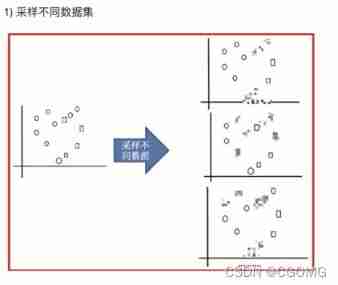
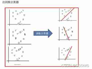
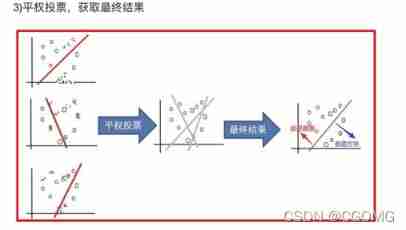
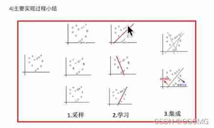
Baggin
Integration principle

Implementation process
Random forest construction process


Interview questions

Out of the bag estimate (Out-of-Bag Estimate)

Definition
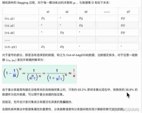

purpose

Random forests API


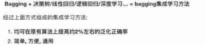
bagging Integration benefits
Random forest case ( Take Titanic passenger survival prediction as an example )
from sklearn.ensemble import RandomForestClassifier
from sklearn.model_selection import GridSearchCV

import pandas as pd
import numpy as np
from sklearn.model_selection import train_test_split
from sklearn.feature_extraction import DictVectorizer
from sklearn.tree import DecisionTreeRegressor,export_graphviz
#  get data
titan = pd.read_csv("titanic.csv")
#  Basic data processing
#  Determine eigenvalue , The target
x = titan[["pclass","age","sex"]]
y = titan["survived"]
#  Missing value processing
x["age"].fillna(value=titan["age"].mean(),inplace=True)
#  Data set partitioning
x_train,x_test,y_train,y_test = train_test_split(x,y,random_state=22,test_size=0.2)
#  Feature Engineering - Dictionary feature extraction
x_train = x_train.to_dict(orient="records")
x_test = x_test.to_dict(orient="records")
transfer = DictVectorizer()
x_train = transfer.fit_transform(x_train)
x_test = transfer.fit_transform(x_test)
#  machine learning - Decision tree
estimator = DecisionTreeRegressor(max_depth=5)
estimator.fit(x_train,y_train)
#  Model to evaluate
print(" score :\n",estimator.score(x_test,y_test))

rf = RandomForestClassifier()
#  Through super parameter tuning
param = {
    "n_estimators":[100,120,300],"max_depth":[3,7,11]}
gc = GridSearchCV(rf,param_grid=param,cv=3)
gc.fit(x_train,y_train)
print(" The result of random forest prediction is :\n",gc.score(x_test,y_test))

otto Case study -Otto Group Product

Data set introduction

Standard for evaluation

Import dependence
import numpy as np
import pandas as pd
import matplotlib.pyplot as plt
import seaborn as sns
from imblearn.under_sampling import RandomUnderSampler
from sklearn.preprocessing import LabelEncoder
from sklearn.model_selection import train_test_split
from sklearn.ensemble import RandomForestClassifier
from sklearn.metrics import log_loss
from sklearn.preprocessing import OneHotEncoder
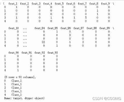
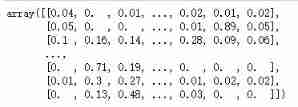
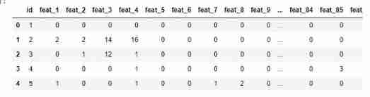
Data acquisition
data = pd.read_csv("train.csv")
data.head()

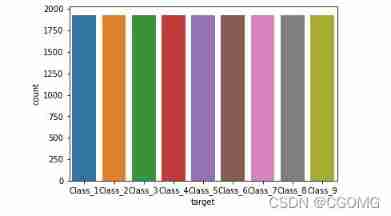
Basic data processing
##  Data categories are uneven
sns.countplot(data.target)
plt.show()

#  Random undersampling to obtain data
##  Determine eigenvalue , The target
y = data["target"]
x = data.drop(["id","target"],axis=1)
x.head(),y.head()
##  Under sampling data acquisition
rus = RandomUnderSampler(random_state=0)
X_resampled,Y_resampled = rus.fit_resample(x,y)
sns.countplot(Y_resampled)
plt.show()
#  Convert tag values to numbers
le = LabelEncoder()
Y_resampled = le.fit_transform(Y_resampled)
#  Split data
x_train,x_test,y_train,y_test = train_test_split(X_resampled,Y_resampled,test_size=0.2,random_state=22)
x_train.shape,y_train.shape,x_test.shape,y_test.shape
model training
##  Open the estimation outside the package
rf = RandomForestClassifier(oob_score=True)
rf.fit(x_train,y_train)
y_pre = rf.predict(x_test)
score = rf.score(x_test,y_test)
rf.oob_score_ #0.7587845622119815
score1 #0.7840483731644111
score
# logloss  Parameter requirements one-hot Format
one_hot = OneHotEncoder(sparse=False)
y_test1 = one_hot.fit_transform(y_test.reshape(-1,1))
y_pre1 = one_hot.fit_transform(y_pre.reshape(-1,1))


log_loss(y_test1,y_pre1,eps=1e-15,normalize=True)
7.4587049513916055
Change the predicted value output mode , Let the output result be percentage , reduce logloss value
y_pre_probae = rf.predict_proba(x_test)
y_pre_probae
rf.oob_score_ #0.7587845622119815
log_loss(y_test1,y_pre_probae,eps=1e-15,normalize=True)
Model tuning
Determine the optimal n_estimators
tuned_parameters = range(10,200,10)
# Create add accuracy One of the numpy
accuracy_t = np.zeros(len(tuned_parameters))
# Create add error One of the numpy
error_t = np.zeros(len(tuned_parameters))
# tuning
for j,one_parameter in enumerate(tuned_parameters):
rf2 = RandomForestClassifier(
n_estimators=one_parameter,
max_depth=10,
max_features=10,
min_samples_leaf=10,
oob_score=True,
n_jobs=-1)
rf2.fit(x_train,y_train)
# Output accuracy
accuracy_t[j] = rf2.oob_score_
# Output log_loss
y_pre_proba = rf2.predict_proba(x_test)
error_t[j] = log_loss(y_test,y_pre_proba,eps=1e-15,normalize=True)
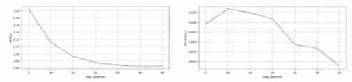
# Visualization of optimization results
fig,axes = plt.subplots(nrows=1,ncols=2,figsize=(20,4),dpi=100)
axes[0].plot(tuned_parameters,error_t)
axes[1].plot(tuned_parameters,accuracy_t)
axes[0].set_xlabel("n_estimators")
axes[0].set_ylabel("errot_t")
axes[1].set_xlabel("n_estimators")
axes[1].set_ylabel("accuracy_t")
axes[0].grid(True)
axes[1].grid(True)
plt.show()

From the image we can see , determine n_estimators=170 When , Good performance
Determine the optimal max_features
tuned_parameters = range(5,40,5)
#  Create add accuracy One of the numpy
accuracy_t = np.zeros(len(tuned_parameters))
#  Create add error One of the numpy
error_t = np.zeros(len(tuned_parameters))
#  tuning
for j,one_parameter in enumerate(tuned_parameters):
    rf2 = RandomForestClassifier(
        n_estimators=170,
        max_depth=10,
        max_features=one_parameter,
        min_samples_leaf=10,
        oob_score=True,
        n_jobs=-1)
    rf2.fit(x_train,y_train)
    #  Output accuracy
    accuracy_t[j] = rf2.oob_score_
    #  Output log_loss
    y_pre_proba = rf2.predict_proba(x_test)
    error_t[j] = log_loss(y_test,y_pre_proba,eps=1e-15,normalize=True)

#  Visualization of optimization results
fig,axes = plt.subplots(nrows=1,ncols=2,figsize=(20,4),dpi=100)

axes[0].plot(tuned_parameters,error_t)
axes[1].plot(tuned_parameters,accuracy_t)

axes[0].set_xlabel("max_features")
axes[0].set_ylabel("errot_t")
axes[1].set_xlabel("max_features")
axes[1].set_ylabel("accuracy_t")

axes[0].grid(True)
axes[1].grid(True)

plt.show()
From the image we can see , determine max_features=15 When , Good performance
Determine the optimal max_depth
tuned_parameters = range(10,100,10)
# Create add accuracy One of the numpy
accuracy_t = np.zeros(len(tuned_parameters))
# Create add error One of the numpy
error_t = np.zeros(len(tuned_parameters))
# tuning
for j,one_parameter in enumerate(tuned_parameters):
rf2 = RandomForestClassifier(
n_estimators=170,
max_depth=one_parameter,
max_features=15,
min_samples_leaf=10,
oob_score=True,
n_jobs=-1)
rf2.fit(x_train,y_train)
# Output accuracy
accuracy_t[j] = rf2.oob_score_
# Output log_loss
y_pre_proba = rf2.predict_proba(x_test)
error_t[j] = log_loss(y_test,y_pre_proba,eps=1e-15,normalize=True)
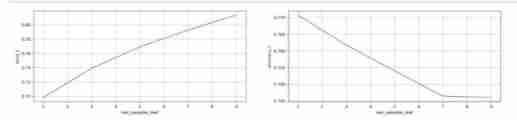
# Visualization of optimization results
fig,axes = plt.subplots(nrows=1,ncols=2,figsize=(20,4),dpi=100)
axes[0].plot(tuned_parameters,error_t)
axes[1].plot(tuned_parameters,accuracy_t)
axes[0].set_xlabel("max_depth")
axes[0].set_ylabel("errot_t")
axes[1].set_xlabel("max_depth")
axes[1].set_ylabel("accuracy_t")
axes[0].grid(True)
axes[1].grid(True)
plt.show()

From the image we can see , determine max_depth=30 When , Good performance
Determine the optimal min_samples_leaf
tuned_parameters = range(1,10,2)
#  Create add accuracy One of the numpy
accuracy_t = np.zeros(len(tuned_parameters))
#  Create add error One of the numpy
error_t = np.zeros(len(tuned_parameters))
#  tuning
for j,one_parameter in enumerate(tuned_parameters):
    rf2 = RandomForestClassifier(
        n_estimators=170,
        max_depth=30,
        max_features=15,
        min_samples_leaf=one_parameter,
        oob_score=True,
        n_jobs=-1)
    rf2.fit(x_train,y_train)
    #  Output accuracy
    accuracy_t[j] = rf2.oob_score_
    #  Output log_loss
    y_pre_proba = rf2.predict_proba(x_test)
    error_t[j] = log_loss(y_test,y_pre_proba,eps=1e-15,normalize=True)

#  Visualization of optimization results
fig,axes = plt.subplots(nrows=1,ncols=2,figsize=(20,4),dpi=100)

axes[0].plot(tuned_parameters,error_t)
axes[1].plot(tuned_parameters,accuracy_t)

axes[0].set_xlabel("min_samples_leaf")
axes[0].set_ylabel("errot_t")
axes[1].set_xlabel("min_samples_leaf")
axes[1].set_ylabel("accuracy_t")

axes[0].grid(True)
axes[1].grid(True)

plt.show()
From the image we can see , determine min_samples_leaf=1 When , Good performance
Determine the optimal model
rf3 = RandomForestClassifier(
    n_estimators=170,
    max_depth=30,
    max_features=15,
    min_samples_leaf=1,
    oob_score=True,
    random_state=40,
    n_jobs=-1)
rf3.fit(x_train,y_train)

rf3.score(x_test,y_test) #0.788367405701123
rf3.oob_score_ #0.7647609447004609
y_pre_probal = rf3.predict_proba(x_test)
log_loss(y_test,y_pre_probal) #0.6964344507957512
Generate submission data
test_data = pd.read_csv("test.csv")
test_data.head()
test_data_drop_id = test_data.drop(["id"],axis=1)
test_data_drop_id.head()

y_pre_test = rf3.predict_proba(test_data_drop_id)
y_pre_test

result_data = pd.DataFrame(y_pre_test,columns=["Class_"+str(i) for i in range(1,10)])
result_data.head()

result_data.insert(loc=0,column="id",value=test_data.id)
result_data.head()

result_data.to_csv("submissson.csv",index=False)
Boosting

Implementation process


baggin Integration and boosting The difference between integration
- difference ⼀: data ⽅⾯
- Bagging: Enter... Into the data ⾏ Sampling training ;
- Boosting: According to the former ⼀ The importance of adjusting data for round learning results .
- difference ⼆: vote ⽅⾯
- Bagging: Equal voting for all learners ;
- Boosting: Go to the learner ⾏ Weighted voting .
- Difference three : Learning order
- Bagging Learning is and ⾏ Of , Each learner has no dependencies ;
- Boosting Learning is a string ⾏, There is a sequence of learning .
- Difference 4 : The main work is ⽤
- Bagging The main ⽤ Yuti ⾼ Generalization performance ( Solve over fitting , It can also be said to reduce ⽅ Bad )
- Boosting The main ⽤ Yuti ⾼ Training accuracy ( solve ⽋ fitting , It can also be said to reduce the deviation )
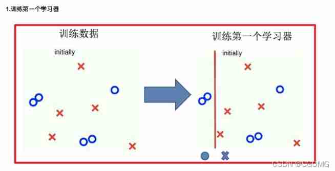
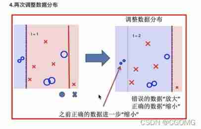
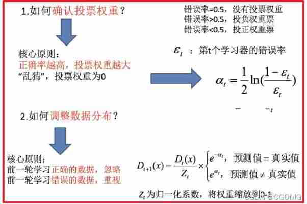
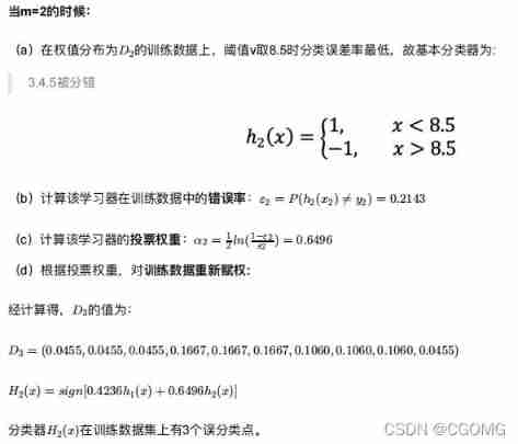
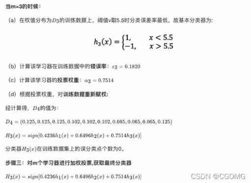
AdaBoost( understand )
Construction process

Case study


API

GBDT( understand )

Decision Tree: CART Back to the tree

Gradient Boosting: Fit negative gradient

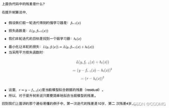
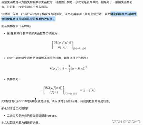
principle

边栏推荐
- 商城系统搭建完成后需要设置哪些功能
- Integration of Android high-frequency interview questions (including reference answers)
- FISCO bcos zero knowledge proof Fiat Shamir instance source code
- Which code editor is easy to use? Code editing software recommendation
- After job hopping at the end of the year, I interviewed more than 30 companies in two weeks and finally landed
- [set theory] binary relation (example of binary relation on a | binary relation on a)
- [literature reading] sparse in deep learning: practicing and growth for effective information and training in NN
- X-ray normal based contour rendering
- [set theory] binary relationship (special relationship type | empty relationship | identity relationship | global relationship | divisive relationship | size relationship)
- Drf--- quick start 01
猜你喜欢

2022 Shandong Province safety officer C certificate examination content and Shandong Province safety officer C certificate examination questions and analysis

Joint search set: the number of points in connected blocks (the number of points in a set)

Introduction of pointer variables in function parameters
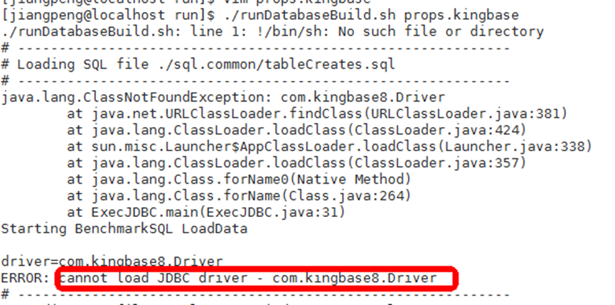
使用BENCHMARKSQL工具对kingbaseES执行灌数据提示无法找到JDBC driver

A outsourcing boy's mid-2022 summary

消息队列(MQ)介绍

Busycal latest Chinese version

Internationalization and localization, dark mode and dark mode in compose

The time has come for the domestic PC system to complete the closed loop and replace the American software and hardware system
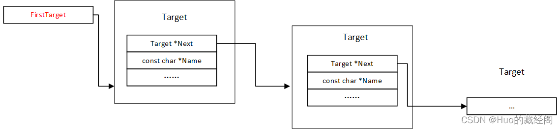
MC Layer Target
随机推荐
arthas watch 抓取入参的某个字段/属性
Why should programmers learn microservice architecture if they want to enter a large factory?
When using the benchmarksql tool to test the concurrency of kingbasees, there are sub threads that are not closed in time after the main process is killed successfully
Xrandr modify resolution and refresh rate
Solve BP Chinese garbled code
Use the benchmarksql tool to perform a data prompt on kingbases. The jdbc driver cannot be found
Bugku CTF daily question baby_ flag. txt
Preliminary cognition of C language pointer
When using the benchmarksql tool to preheat data for kingbasees, execute: select sys_ Prewarm ('ndx_oorder_2 ') error
[pat (basic level) practice] - [simple simulation] 1063 calculate the spectral radius
Contents of welder (primary) examination and welder (primary) examination in 2022
Design and implementation of JSP logistics center storage information management system
Function introduction of member points mall system
What's wrong with SD card data damage? How to recover SD card data damage
540. Single element in ordered array
Internationalization and localization, dark mode and dark mode in compose
[set theory] inclusion exclusion principle (including examples of exclusion principle)
2022-02-14 (394. String decoding)
Sklearn data preprocessing
FFMpeg example