[day1/5 literature intensive reading] speed constancy or only slowness: what drives the kappa effect

Read the literature ：

Chen Y, Zhang B, Kording KP (2016) Speed Constancy or Only Slowness: What Drives the Kappa Effect. PLoS ONE 11(4): e0154013. doi:10.1371/journal.pone.0154013

Links to Literature ：Speed Constancy or Only Slowness: What Drives the Kappa Effect

List of articles

• Abstract
• One 、 Preface
• Two 、 Experiment 1
• 1、 Experimental design
• 2、 Bayesian model
• 3、 Fit the model to the data fitting
• 3、 ... and 、 Experiment two
• 1、 Experimental design
• 2、 experimental result
• Four 、 Discuss

---

Abstract

What is? Kappa effect ： The effect of spatial distance on time perception

Two model assumptions ： Classic models （ Constant speed ）VS Bayesian model （ Slow speed a priori ）

        → The visual experiment in this paper finds that ：

        1） When fitting data, both models can replicate the subjects' reactions , But Bayesian models are better at predicting behavior ;

        2） The estimated constant velocity is close to the absolute threshold of velocity ;

        3）Kappa The effect is caused by slow speed , And regulated by spatial variability .

---

One 、 Preface

1、Kappa Effect explanation ： Quote examples , When two objects appear in succession at a constant time interval , The greater the space interval, the greater the perceived time interval .

2、 Classic models （Classical model） Introduce ： The object moves at a constant speed in the background , Perceiving （ It is estimated that ） The time interval between the appearance of two objects (estimated time) te By the sample interval (sample time) ts And the expected time E(t)（ Given distance l/ Constant speed v0） weighting （ The weight of ω） have to ：

           ( Eq1)

However ,ω It is unknown. .

3、 Bayesian model （Bayesian model, It is also expressed as a slow speed model Slowness model） Introduce ： The object moves slowly in the background , It has been reproduced in a series of tactile spatiotemporal perception tasks Kappa effect , But can it explain vision Kappa The effect has yet to be tested .

4、 In this paper, ：

Bayesian model ： A posteriori mean = Weighted average of prior and likelihood means ;

In the classical model ： Perceived time = Weighted average of actual time and expected time ;

       →  This may indicate ： Under the appropriate definition , Classical models can also be expressed in the form of Bayesian models .

5、 This paper assumes that ： The subjects thought that the object was moving at a constant speed ;

Research methods ： Bayesian model is used to describe the slow speed model and classical model , Perform a time copy task to reproduce the vision Kappa effect

research objective ： Explore which model can better explain Kappa effect .

---

Two 、 Experiment 1

1、 Experimental design

9 Subjects participated in 17（ Horizontal distance between two circles ）×2（ Time interval between two circles sample time interval,0.8s/1.2s） In subject experiment design , Press the key to copy the time interval between two circles (producted time) tp, Each process 40 individual trail common 1360 individual trail.

2、 Bayesian model

（1） For classical models ： The time interval between the occurrence of two circles is estimated by the subjects  te See Eq1.

The classical model is expressed in the form of Bayesian model , The process is as follows ：

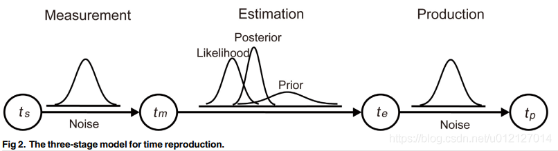
The construction of Bayesian model is divided into three stages , An ideal observer model reproduced by time ideal observer model for time reproduction modified , Here's the picture ：

Sort out the symbols and concepts involved in this part ：

ts	Sample time sample time	Time interval between actual presentation of samples
tm	Measuring time measured time（ Distribution ）	The time measured by the subject for the sample time interval , To obey the mean is ts The standard deviation is σm Gaussian distribution of , Write it down as p(tm|ts), It can be regarded as the time of feeling registration / Sensory memory representation
te	Estimate the time estimated time	According to Bayesian model , combination prior And likelihood Estimated time obtained , yes posterior The average of , It can be regarded as the time of perception
tp	Copy time producted time（ Distribution ）	In the reaction phase, the subjects press the key to copy the time distribution , Write it down as p(tp|te)
prior	transcendental （ Distribution ）	Previous experience of the velocity of a body moving at a uniform speed , To obey the mean is l/v0 The standard deviation is στ Gaussian distribution of , remember p(τ)
likelihood	Likelihood （ Distribution ）	To obey the mean is τ The standard deviation is σm Gaussian distribution of , Write it down as p(tm|τ),τ Time for experience is also a Gaussian distribution . In my submission likelihood According to the experience time τ Measured time obtained tm The distribution of .
posterior	Posttest （ Distribution ）	combination prior And likelihood The resulting distribution , The mean for te

Bayes' rule ：

P(A|B)=P(B|A)*P(A)/P(B)
→ It can also be rewritten as ： Posterior probability ∝ Likelihood * Prior probability     (∝ It means that two numbers are in direct proportion )
    Reference resources ： No basic understanding of Bayes - The evening moon bends - Blog Garden

        1）Measurement： Sample interval ts Measured by subjects ; In the given ts Under the condition of , The time interval measured by the subjects tm The distribution of is p(tm|ts), Its mean value is ts The standard deviation is σm Gaussian distribution of . This is related to Scalar timing theory scalar timing theory Agreement （ The internal characterization of time interval is the distribution of multiple values with accurate mean value ）.

        2）Estimation： The constant velocity of a moving object v0 Have a priori belief , At a given moving distance l Under the condition of , Subjects will have a prior time interval distribution p(τ), Its mean value is l/v0 The standard deviation is στ Gaussian distribution of , as follows ：
                   ( Eq2)

The likelihood is p(tm|τ), To obey the mean is τ The standard deviation is σm Gaussian distribution of , Then the posterior distribution can be calculated by Bayes rule ：

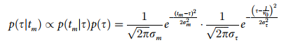          ( Eq3)

  The mean value of the posterior distribution （ The estimated time interval of the subjects  te） by ：

          ( Eq4)

See Day 37 Read the literature ：Körding, K. P., & Wolpert, D. M. (2006). Bayesian decision theory in sensorimotor control. trends in cognitive sciences, 10(7), 319-326.

The combination (posterior) of likelihood and prior in Bayes’ rule is driven by their respective uncertainty (variance).

Given sample interval ts, Then the estimated time interval of the subjects  te by ：

    ( Eq5)

Make   , Then there are ：

               ( Eq6)

so , The time interval estimated by the subjects is calculated by Bayesian model  te Of Eq6 And classical model calculation te Of Eq1 equal , explain Eq1 It can be defined as a Bayesian model .

         3）Production： The subjects used the estimated time interval  te To press the key to copy tp, In the given te Under the condition of ,tp The distribution of is p(tp|te). Previous studies have shown that （ Here we also need to look at the references ）,tp The standard deviation increases linearly with its mean , This feature is called Scalar variability , namely scalar variability. therefore σp=wp*te,wp It's a Weber score Weber fraction, Then there are ：

                 ( Eq7)

 （2） For the slow speed model ：Goldreich To reproduce the sense of touch Kappa A Bayesian model based on the assumption of slow speed , Defined as having a center of 0 Gaussian distribution function of , Its derivation Kappa The formula of the effect Eq8. The derivation process is as follows ：

        1） The slow velocity model is based on the probability distribution of neural activity , A tactile stimulus on the skin will evoke a neural response D. The given initial tactile stimulus position is x1, The neural activity of arousal can be modeled as spatial location x Function of , Its mean value is x1 Gaussian distribution of ：

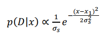                  ( A7 )

        2）  The given position of the second tactile stimulus is x2, The velocity and time interval between the two stimuli were v and τ, Then the neural probability distribution of the second tactile stimulation is ：

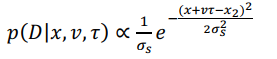      ( A8 )

        4） Neural activity can also be modeled as time t The Gauss function of , The center is the time when the real tactile stimulus is applied . The actual application time of the first tactile stimulus is defined as 0, The second time is ts（ That is, the time interval between two stimuli ）, Then the Gaussian distributions of the two neural activities with respect to time are ：

                      ( A9 )

                     ( A10 )

        5） The likelihood of generating neural activity between two stimuli likelihood Can be written as space x And time t Probability distribution of ：

      ( A11 )

        6） Slow speed a priori prior It reflects the expectation of slow motion , It is modeled as having a mean of 0 The Gauss function of ：

                        ( A12 )

        7） So according to A11 and A12, A posteriori distribution can be calculated using Bayesian rules ：

                       ( A13 )

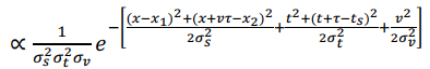
        8） take A13 The exponent of x、v、t and τ The partial derivative of is set to 0 A posteriori pattern is obtained , Perceived time te In a posteriori mode τ Value , be ts And te The relation of is （ This step is not very clear ）：

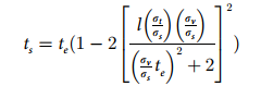                 ( Eq8)

among ,l Is the distance between two stimuli ,ts Is the sample interval ,te The estimated time interval for the subjects ,σs and σt Are the standard deviations of perceived spatial and temporal information respectively ,σv Is the standard deviation of a priori velocity .

Last , The subjects used te To press the key Copy the time interval between two circles tp, This process is similar to the third step in the Bayesian version of the classical model production Agreement .

3、 Fit the model to the data fitting

Assume with any ts dependent tp The value is independent in the experiment . all N Of individuals in trials tp The joint conditional probability of values joint conditional probability by ：

         ( Eq9)

After logarithm, we get ：

         ( Eq10)

（1） Model parameters parameters：matlab The maximum likelihood method maximizing the likelihood determine , Previous studies have shown that ω Is a function of the sample time interval （ Here we also need to look at the references ）, Therefore, the classical model includes 4 Parameters ,ω0.8（0.8s Weight in time interval condition ）、ω1.2、v0 and wp（ Weber score ）; It is also in the slow speed model 4 Parameters ,σt0.8、σt1.2、σv and wp.

（2） Calculation σs Methods （σs It's not a parameter , Can be calculated to obtain ）

        1） Minimum perceptible error JND(just noticeable difference)： In psychometric function 25% and 75% Differences between , Standard deviation (σ) It can be used JND A Gaussian distribution is calculated , namely ：

        σ =JND/0.6475

        2） Visual acuity threshold visual acuity threshold： by JND Application in spatial resolution measurement of visual processing system , Previous studies have reported 2 Visual acuity threshold (Vernier/grating resolutions) As eccentricity eccentricity Function of , Respectively ：

k = 0.93 ×ε^0.69  and  k = 1.34 × ε^0.71  (the unit of κ is minute not degree)
among ,κ Is the visual acuity threshold (JND For spatial resolution ),ε Is eccentricity .

        3） So there is σs Calculation formula ：

σs = 0.0239 × ε^0.69(Vernier resolution) and σs = 0.0345 × ε^0.71(grating resolution),(the unit of σs is degree not minute)
（3）Akaike information criterion (AIC)： It is used to evaluate the fitting degree of the model

Δ = AICi-AICmin
among ,AICi From i A model ,AICmin From the best model （AIC Minimum ）.Δ The smaller it is, the smaller the difference between the model and the best model is , The better the fitting degree of the model .

 3、 experimental result

（1） Research purpose and method ： Which of the constant velocity and slow velocity hypotheses can best explain Kappa effect ？ In the design of this experiment , The time when the test copy occurs tp It can be expressed as a function of the spatial distance between two stimuli and the presentation time distance .

（2） Reaction deviation response bias (BIASr)

        1） Calculation BIASr： stay At each time interval , The two circles are directly above the gaze 30mm At the same position in succession , The replication time of the subjects tp Mean and standard time interval ts The difference between is BIASr.

        2） Single sample t test One sample t-test： stay 0.8s Under the condition of time interval ,BIASr remarkable ＞0（p<0.05）; stay 1.2s Not significant under time interval conditions .

        3）BIASr The significance and correction of ：BIASr It represents the deviation of subjects' response independent of the spatial distance of stimulus presentation , It can be used as a baseline baseline, Although its value is very small , As a corrective , In the analysis, the corresponding reaction deviation was subtracted from the replication time of each subject .

（3）BIASk And VAR： Under each treatment , When two circles appear in the same position ,BIASk Is the replication time of the subject tp Mean and baseline baseline The deviation value of ,VAR Is the corresponding variance , See the picture below ：

        1）BIASk As the space distance between two circles increases （ The distance between the black dot and the green line increases from left to right ）;

        2） For all subjects ,VAR stay 0.8s Significant at time intervals ＜1.2s Time interval （p<0.05）（A Grey dot ratio in the figure B The picture is more concentrated ）, It means that there is more uncertainty in copying a longer sample , This is related to Scalar variability Agreement .

（4） Fitting data ： Both the classical model and the slow speed model can reproduce the results of the subjects （ The fitting curve basically coincides with the black spot ）, Here's the picture ：

        1） Classic models ： The production time is predicted as a linear function of distance . Mean value of model parameters ,ω0.8 and ω1.2 Very close to 1,v0 about 0.2°/s, wp about 0.2, See the table below ：

         2） Slow speed model ： stay 0.8s Under the condition of time interval , It is estimated that the growth rate over a long distance will be slower than that over a short distance , It is closer to the result of slow speed model ; stay 1.2s Under the condition of time interval , It is close to the results of both models . stay 2 In the case of threshold limit values of visual acuity , The estimated time is almost the same （Fig 4B And 4C The fitting curves in are almost the same ）, And the best fitting parameters are almost the same （ The following table ）,  stay 0.8s and 1.2s Under the condition of time interval σt Respectively about 0.01s and 0.02s,σv about 0.9°/s,wp about 0.2.

         3） from Fig 4, The slow speed model seems to better explain the data qualitatively （ Better predict behavior ）.

（5）AIC difference (Δ)： The empirical criterion for the degree of model fitting is 0≤Δ ≤2, substantial; 4 ≤ Δ ≤7, considerably less; Δ >10, essentially none. The results are shown in the table below ：

        1） For the slow speed model , stay 0.8s Under the condition of time interval ,6 The fitting degree of subjects is significantly better than the classical model , And in the 1.2s Under the condition of time interval, only 1 individual （ The green part of the table ）;

        2） Symbol test sign test indicate , stay 0.8s Under the condition of time interval, the fitting degree of slow velocity model is better (p < 0.01), and 1.2s Under the condition of time interval, the difference of fitting degree between the two models is not significant (p > 0.05).

 （6） The prediction of the model ： Use best fit parameters the best-fitting parameters The prediction of the two models over a longer range is plotted as follows （ The visual acuity threshold of the slow speed model only uses Vernier resolution）：

        1） Classic models ： The replication time increases linearly with distance ;

        2） Slow speed model ： The replication time increases linearly with distance , But the growth rate tends to slow down ;

        3） The difference between the two models increases with distance . This shows that in the future Kappa In effect study , Need to use a larger distance range .

---

3、 ... and 、 Experiment two

There is a basic assumption in Experiment 1 ： The subjects are A sample time （ Time interval between two circles ） There is only one reaction deviation . The purpose of this experiment is to supplement and verify whether the response bias is affected by the location of stimulus presentation .

1、 Experimental design

9 Name of subjects （ Different from Experiment 1 ） Participate in 3（ The positions of the two circles are the same , The horizontal distance from the fixation point is left 12°/0°/ Right 12°）×2（ Time interval between two circles sample time interval,0.8s/1.2s） In subject experiment design , Press the key to copy the time interval between two circles , Each process 40 individual trail common 240 individual trail.

2、 experimental result

Response deviation of each subject at each time interval and each presentation position response biases (BIASr) Of M and SE The following table ：

Yes 3 Location 、2 Two factor repeated measurement design analysis of variance was done for each time interval Two-way repeated measurement ANOVA： Time interval 、 Location 、 The main effect of the interaction between time distance and position main effects Are not significant （p ＞ 0.05）, This indicates that the position of stimulus presentation has no significant effect on response bias .

---

Four 、 Discuss

（1） In experiment one , By comparing the model fitting, it is found that , Both the classical model based on the constant velocity hypothesis and the slow velocity model based on the slow velocity can reproduce the subjects' responses （Fig 4）, but AIC The index shows that the slow speed model can better fit the data .

（2） About the reaction bias found in this study response bias

        1） There has been no previous study on whether the presentation position of visual stimuli has an impact on response bias , In Experiment 2, we found that , The result was no significant effect ;

        2） In the classical model ,Jones and Huang Put forward at a given time interval the given duration(ts), Given distance (l),Kappa Effect calculation (A4) branch 3 Step ：

        ① adopt psychophysical function：φt, take ts Into it scale value ：

                   (A1)

        ②  Internal code of observation time internal code It can be expressed as scale value And expected time expected time Weighted form of ：

                       (A2)

        among , Expect time E(t)=l/v0,v0 It's a constant speed . 

        ③  adopt psychomotor function：ht, utilize internal code Get the copy time tp：

                  (A3)

        Jones and Huang Think φt Is linear , Can make ：

                among Represents deviation , be A2 Can be written as ：

                (A4)

        It can be seen that ,Jones and Huang The reaction deviation is not clearly indicated . But in Experiment 1 of this study , By defining the reaction deviation ：, The reaction deviation is separated from the sample time (Fig 3),A4 Can be written as ：

           (A5)

        Take the data BIASr After correction ：

                             (A6)

         A6 And Jones and Huang It is concluded that the Kappa Effect equation A4 Mathematically equivalent , But it has more definite psychological significance .

（3） Model fitting data 2 Methods

        1） Correct the reaction deviation before fitting the data , Determine baseline levels . This is also the method used in Experiment 1 of this study .

        2） Take the reaction deviation as the parameter of the model , Fit the data . Through supplementary analysis, it is found that , This method makes the parameters of the two models change from the original 4 The number is increased to 6 individual （ newly added BIASr0.8 and BIASr1.2, We can see the equation A5）, This may lead to over fitting when fitting some of the tested data overfitting The phenomenon .

（4） On the assumption of slow speed

        1） Slow speed model ： Based on a priori velocity assumption , And the prior speed is slow , The center is 0;

        2） Classic models ： Also based on a priori velocity assumption , And the prior velocity is a constant velocity , Logically speaking , This constant speed can also be a slow speed , For the following reasons ：

        ①  from Fig 2, Posteriori time posterior The mean of is greater than the likelihood likelihood The average of , Then the mean of a priori time must be greater than the likelihood （ Because a posteriori is a combination of a priori and likelihood ）, That is, a priori speed is slower than the speed of stimulus circle flash (v = l/t); In Experiment 1, a constant velocity is obtained v0 about 0.2°/s, It's much slower than the flash of a circle (1.2 to 28.3°/s);

        ② Previous studies have shown that , The absolute speed threshold of the aged subjects is 0.12°/s, The young subjects were 0.09°/s, And v0 near , Therefore, it is reasonable to regard constant speed as slow speed , This is also the reason why both the classical model and the slow speed model reproduce the reaction of the subjects (Fig 2);

        ③  The slow speed Apriori is proved to reflect the statistical structure of the visual environment , That is, there are relatively few fast-moving objects , But it's The neural mechanism of the occurrence needs further study ;

（5） The two models fit the data

        1） from Fig 4, The slow speed model only 0.8s Under these conditions, the growth rate tends to slow down ,1.2s The reason why the condition does not appear is that the distance between the two circles is not long enough 1.4° to 22.6°. from Fig 5, The distance increased to 1.4° to 150° after , The slow speed model is 1.2s Under these conditions, the growth rate has also slowed down .

        2） The slow speed model shows a trend of slow growth under long-distance conditions , The classical model is linear , The data fitting ability of slow speed model is better .

        3） Why does the slow speed model show a slowdown trend in growth over a long distance ？

        → The slow velocity model takes into account the spatial variability spatial variance, The greater the value → Eccentricity eccentricity The bigger it is → Visual acuity visual acuity The lower the → The shorter the perceived distance → The shorter the perceived time span

（6） The advantages and disadvantages of the two models

        1） Classic models

        advantage ： Based on a simple linear model ;

        shortcoming ：

        ①  Poor data fitting ability , The nonlinear characteristics of spatial information are not considered （ Such as spatial variability ）;

        ②  The weight in the model ω Change with sample time , This makes it impossible for the model to predict the replication time of a new sample time with the obtained best fitting parameters .

        2） Slow speed model

        advantage ： Probability distribution based on neural activity , Considering the uncertainty of spatiotemporal information , It is predicted that the replication time will slow down as the distance increases , The ability to fit data is stronger ;

        shortcoming ：

        ①  The model representation is complex , Estimated time cannot be written as a function of sample time te = f(ts), Therefore, it is impossible to obtain accurate te.

        ②  The value of spatial variability comes from the calculation of previous studies , And keep the same for all subjects , But it may be due to the individual differences of the subjects 、 Brightness contrast and other reasons .

        ③  The uncertainty of time information changes with the change of sample time , This makes it impossible for the model to predict the replication time of a new sample time with the obtained best fitting parameters .

therefore , To build a better Kappa Effect model , The advantages and disadvantages of the slow speed model and the classical model should be considered .