当前位置:网站首页>CV learning notes - image filter
CV learning notes - image filter
2022-07-03 10:07:00 【Moresweet cat】
Image filter
1. Image filtering
1. Image filtering & filter
Image filtering : That is to suppress the noise of the target image while preserving the details of the image as much as possible , It is an indispensable operation in image preprocessing , The quality of its processing effect will directly affect the effectiveness and reliability of subsequent image processing and analysis .
filter : Think of the filter as a lens with weighting coefficients , When using this filter to smooth the image , Is to put this lens on the image , Look at the image we get through the lens .
2. The purpose of image filtering is & requirement
Filtering purpose :
- Eliminate the noise in the image .
- Extract image features for image recognition .
Filtering requirements :
- Do not damage the image outline and edges .
- The visual effect of the image should be better .
3. Filter type
- Linear filtering
Linear filtering is the most basic method of image processing , Directly use the filter to process the image , According to the filter matrix elements , Can produce many different effects .
![[ Failed to transfer the external chain picture , The origin station may have anti-theft chain mechanism , It is suggested to save the pictures and upload them directly (img-gYYTGJqx-1638773250584)(./imgs/image-20211127161452417.png)]](/img/5f/126f0c9c1604dbe99092956d0e6711.jpg)
- Mean filtering
The ideal mean filtering is to replace each pixel in the image with the average value calculated by each pixel and its surrounding pixels . It is very commonly used in image processing , From the point of view of frequency domain, mean filtering is a low-pass filter , High frequency signals will be filtered and eliminated after processing , Because of this feature , Mean filtering is often used to eliminate image sharp noise , Achieve image smoothing 、 Fuzzy and other functions .
g ( x , y ) = 1 M ∑ f ∈ s f ( x , y ) g(x,y)=\frac{1}{M}\sum_{f\in{s}}f(x,y) g(x,y)=M1f∈s∑f(x,y)
Algorithm flow :
1.  Each pixel in the image is calculated from left to right and from top to bottom , Finally, the processed image .
2.  Two parameters can be added to the mean filter , The number of iterations ,Kernel data size .
3.  One of the same Kernel, But many iterations will get better and better .
4.  Again , Same number of iterations ,Kernel The larger the matrix , The more obvious the effect of mean filtering .
![[ Failed to transfer the external chain picture , The origin station may have anti-theft chain mechanism , It is suggested to save the pictures and upload them directly (img-IoWxOwFA-1638773250586)(./imgs/image-20211127163240533.png)]](/img/a1/c4945ad7f2f7f33dd8d94466b457bb.jpg)
advantage : Method is simple , Fast calculation .
shortcoming : Reduce noise and blur the image , Especially the edges and details of the scene .
- median filtering
The median filter replaces the central pixel with the median after sorting the surrounding pixel and the central pixel , The effect of median filtering is often better than that of mean filtering , Especially to eliminate salt and pepper noise .
![[ Failed to transfer the external chain picture , The origin station may have anti-theft chain mechanism , It is suggested to save the pictures and upload them directly (img-Q53hOyU1-1638773250586)(./imgs/image-20211127163848801.png)]](/img/62/08e22d01a2e1eb16e0d3c8ec91e8f6.jpg)
advantage : The inhibition effect is very good , The clarity of the picture is basically maintained ;
shortcoming : The effect of suppressing Gaussian noise is not very good .
- Maximum and minimum filtering
The maximum and minimum filter uses the sorted maximum value of surrounding pixels to compare with the minimum value and the central pixel to determine the central replacement pixel , If the central pixel is larger than the maximum , Replace the center pixel with the maximum ; If the central pixel is smaller than the minimum , Then the center pixel is replaced with the minimum value . It is a conservative image processing method .
![[ Failed to transfer the external chain picture , The origin station may have anti-theft chain mechanism , It is suggested to save the pictures and upload them directly (img-wJ61S6gR-1638773250587)(./imgs/image-20211127164426552.png)]](/img/6c/b4ddb24483158ff51e7dea570c816d.jpg)
- Guided filtering
( lead ) Local linear model
A point on a function has a linear relationship with the points of its adjacent parts , A complex function can be represented by many local linear functions , When you need to find the value of a point on the function , Just calculate and average the values of all linear functions containing this point . Local linear models are very helpful in representing non analytic functions .
![[ Failed to transfer the external chain picture , The origin station may have anti-theft chain mechanism , It is suggested to save the pictures and upload them directly (img-Jc2zw6Hq-1638773250589)(./imgs/image-20211128114959667.png)]](/img/04/d0380ecc444ca0d8055021e56c3ee2.jpg)
The two-dimensional image can be regarded as a two-dimensional linear function without an exact analytical expression , Suppose the output and input of the function are in a two-dimensional window Satisfy linear relationship :
q i = a k I i + b k , Yes On whole body i ∈ ω k q_i=a_kI_i+b_k, For all i\in\omega_k qi=akIi+bk, Yes On whole body i∈ωk
among ,q Is the value of the output pixel ,I Is the value of the input image ,i and k Is the pixel index ,a and b When the center of the window is k The coefficient of the linear function . Actually , The input image is not necessarily the image to be filtered, but also the guide image of other images , That's why it's called guided filtering . Take the gradient on both sides of the above formula , You can get :
∇ q = a ∇ I \nabla q=a\nabla I ∇q=a∇I
That is, when inputting an image I With gradient , Output q There are similar gradients , This is also the reason why guided filtering has edge preserving characteristics .
The next step is to find the sparsity of the linear function , That's linear regression , That is, you want to fit the output value with the real value p The gap between them is the smallest , That is to say, let the following formula be the minimum :
E ( a k , b k ) = ∑ i ∈ ω k ( ( a k I i + b k − p i ) 2 + ϵ a k 2 ) E(a_k,b_k)=\sum_{i\in \omega_k}((a_kI_i+b_k-p_i)^2+\epsilon a^2_k) E(ak,bk)=i∈ωk∑((akIi+bk−pi)2+ϵak2)
there p Only images to be filtered , It's not like I That can be other images , meanwhile a The previous coefficient ( Write it down as e) Used to prevent getting a Too big , It is also an important parameter to adjust the filtering effect of the filter . By the least square method , We can get :
a k = 1 ∣ ω ∣ ∑ i ∈ ω k I i p I − μ k p ‾ k σ k 2 + ϵ b k = p ‾ k − a k μ k a_k=\frac{\frac{1}{|\omega|}\sum_{i\in \omega_k}I_ip_I-\mu_k\overline{p}_k}{\sigma^2_k+\epsilon}\\ b_k=\overline{p}_k-a_k\mu_k ak=σk2+ϵ∣ω∣1∑i∈ωkIipI−μkpkbk=pk−akμk
among , μ k \mu_k μk yes I At the window ω k \omega_k ωk The average of , σ k 2 \sigma^2_k σk2 yes I At the window ω k \omega_k ωk Variance in , ∣ ω ∣ |\omega| ∣ω∣ It's the window ω k \omega _k ωk Number of pixels in , p ‾ k \overline{p}_k pk Is the image to be filtered p At the window ω k \omega _k ωk Mean in .
When calculating the linear coefficient of each window , We can see that a pixel is contained in multiple windows , in other words , Each pixel is described by several linear functions . therefore , As I said before , When you want to specify the output value of a certain point , Just average the values of all linear functions containing the point :
q i = 1 ∣ ω ∣ ∑ k : i ∈ ω k a k I k + b k = a ‾ i I i + b ‾ i \begin{aligned} q_i&=\frac{1}{|\omega|}\sum_{k:i\in\omega _k}a_kI_k+b_k\\&=\overline{a}_iI_i+\overline{b}_i \end{aligned} qi=∣ω∣1k:i∈ωk∑akIk+bk=aiIi+bi
here , ω k \omega_k ωk Include all pixels when i The window of ,k It's the center of it .
When the guided filter is used as an edge preserving filter , There is often I = p I=p I=p, If e = 0 e=0 e=0, obviously a = 1 a=1 a=1, b = 0 b=0 b=0 yes E ( a , b ) E(a,b) E(a,b) Is the solution of the minimum , It can be seen from the above formula , The filter doesn't work at all , The input will be the same as the output . If e>0, In areas where pixel intensity changes little ( Or monochromatic areas ), Yes a a a Approximate to ( Or equal to )0, and b b b Approximate to ( Or equal to ), That is to say, we do a weighted mean filter ; And in areas of great change , a a a Approximate to 1, b b b Approximate to 0, The filtering effect on the image is very weak , It helps to keep the edges . and e e e The role of big change is to define what big change is , What is small change . With the same window size , With e e e The increase of , The more obvious the filtering effect is .
2. Image noise
1. summary
Image noise is the random signal interference in the process of image acquisition or transmission , Signals that hinder people's understanding, analysis and processing of images .
The generation of image noise comes from the environmental conditions in image acquisition and the quality of the sensor itself , The main factor of image noise in the transmission process is that the transmission channel used is polluted by noise .
2. Gaussian noise
Definition : Gaussian noise (Gaussian noise) It refers to a kind of noise whose probability density obeys Gaussian distribution .
![[ Failed to transfer the external chain picture , The origin station may have anti-theft chain mechanism , It is suggested to save the pictures and upload them directly (img-HJfrScLh-1638773250591)(./imgs/image-20211206135347911.png)]](/img/35/c8387604e0cee92368b8bd0eb86cf8.jpg)
white Gaussian noise : Noise whose amplitude obeys Gaussian distribution is uncorrelated between any two sampled samples .
White noise : Uncorrelated noise between any two sampled samples .
Cause of occurrence :
- The image sensor is not bright enough when shooting 、 Uneven brightness ;
- The noise and mutual influence of each component of the circuit ;
- The image sensor works for a long time , The temperature is too high ;
Add Gaussian distribution :
- Input parameters sigma and mean
- Generate Gaussian random number
- The output pixel is calculated from the input pixel
- Zoom all pixel values back to [0~255] Between
- Cycle through all pixels
- Output image
A normal Gaussian sampling distribution formula , Get the output pixels Pout
Pout = Pin + random.gaussamong random.gauss It's through sigma and mean To generate random numbers that conform to the Gaussian distribution .
3. Salt and pepper noise
Definition : Salt and pepper noise is also called impulse noise , It is a random white dot or black dot .
Pepper noise & Salt noise : Pepper noise (pepper noise)+ Salt noise (salt noise). The value of salt and pepper noise is 0( Any of several hot spice plants ) perhaps 255( salt ). The former is low gray noise , The latter belongs to high gray noise . Generally, two kinds of noise appear at the same time , Black and white specks appear on the image . For color images , It may also appear in a single pixel BGR Three channels appear randomly 255 or 0.
The reasons causing : If there is an error in communication , Some pixel values are lost during transmission , This noise will occur . The cause of salt and pepper noise may be the sudden strong interference of the image signal . For example, a failed sensor results in a minimum pixel value , Saturated sensors result in maximum pixel values .
Add salt and pepper noise :
- Specify the signal-to-noise ratio SNR( The proportion of signal and noise ) , Its value range is [0, 1] Between
- Calculate the total number of pixels SP, Get the number of pixels to noise NP = SP * SNR
- Randomly get every pixel position to be noisy P(i, j)
- Specify the pixel value as 255 perhaps 0.
- repeat 3, 4 Complete all... In two steps NP Pixel noise
4. Other noise
Poisson noise : A noise model with Poisson distribution , Poisson distribution is suitable to describe the probability distribution of the number of random events in unit time . For example, the number of service requests received by a service facility in a certain period of time , The number of calls received by the telephone exchange 、 The number of people waiting at the bus platform 、 The number of machine failures 、 The number of natural disasters 、DNA The number of variations in the sequence 、 Decay number of radioactive nuclei, etc .
characteristic :
- The longer the time , The more likely an event is to occur , And the probability of this event occurring at different times is independent of each other
- For a very short period of time , The probability of this time occurring twice is almost zero
- At the beginning, the incident did not happen
P { ( N ( t + τ ) − N ( t ) ) } = e − λ τ ( λ τ ) k k ! k = 0 , 1... P\{(N(t+\tau)-N(t))\}=\frac{e^{-\lambda\tau}(\lambda\tau)^k}{k!}\quad k=0,1... P{ (N(t+τ)−N(t))}=k!e−λτ(λτ)kk=0,1...
Multiplicative noise : It is generally caused by the imperfect channel , The relationship between them and signals is multiplication , The signal is there. It's there , If the signal is not there, he will not be there .
rayleigh noise : Compared with Gaussian noise , Its shape is skewed to the right , This is useful for fitting some skew histogram noise . Rayleigh noise can be realized by average noise .
Gamma Noise : Its distribution obeys the distribution of gamma curve . Realization of gamma noise , Need to use b A noise subject to exponential distribution is superimposed . Exponentially distributed noise , Uniform distribution can be used to achieve .(b=1 Is exponential noise ,b>1 Through the superposition of several exponential noises , Get gamma noise )
3. Image enhancement
1. summary
Purposefully emphasize the overall or local characteristics of the image , Make the original unclear image clear or emphasize some interesting features
sign , Expand the difference between different object features in the image , Suppress features that are not of interest , Make it improve the image quality 、 Enrich
The amount of information , Enhance the image interpretation and recognition effect , Meet the needs of some special analysis .
There are two types of image enhancement :
- Point processing technology . Only a single pixel is processed .
- Neighborhood processing technology . Processing pixel points and points around them , That is, using convolution kernel .
2. Do something about it
1. linear transformation
effect : Image enhancement linear transformation is mainly to adjust the contrast and brightness of the image :
y = a x + b y=ax+b y=ax+b
Parameters a a a Affect the contrast of the image , Parameters b Affect the brightness of the image , It can be divided into the following situations :
- a > 1 a>1 a>1: Enhanced the contrast of the image , The image looks clearer .
- a < 1 a<1 a<1: Reduces the contrast of the image , The image looks blurred
- a = 1 & & b ≠ 0 a=1\&\&b\neq0 a=1&&b=0: The gray value of the whole image moves up or down , That is to say, the whole image becomes bright or dark , Does not change the contrast of the image , b > 0 b>0 b>0 Image lightens when , b < 0 b<0 b<0 The image darkens when .
2. Piecewise linear transformation
effect : In a given interval x Inside , Make a linear transformation , Adjust the contrast coefficient , Increase or decrease the contrast in the area .
{ y = a 1 x + b x < x 1 y = a 2 x + b x 1 < x < x 2 y = a 1 x + b x 2 < x \left\{ \begin{aligned} y&=a_1x+b\quad x<x_1\\ y&=a_2x+b\quad x_1<x<x_2\\ y&=a_1x+b\quad x_2<x \end{aligned} \right. ⎩⎪⎨⎪⎧yyy=a1x+bx<x1=a2x+bx1<x<x2=a1x+bx2<x
3. Logarithmic transformation
effect : Logarithmic transformation expands the low gray value part of the image , Compress its high gray value part , In order to emphasize the low gray part of the image ; At the same time, it can well compress the dynamic range of the image with large changes in pixel values , The purpose is to highlight the details we need .
y = c ∗ l o g ( 1 + x ) y=c*log(1+x) y=c∗log(1+x)![[ Failed to transfer the external chain picture , The origin station may have anti-theft chain mechanism , It is suggested to save the pictures and upload them directly (img-zI7uxBph-1638773250592)(./imgs/image-20211206143045087.png)]](/img/7e/c5f6e3d3879de77899de4e78f3c926.jpg)
4. Power law transformation / Gamma transform
effect : Power law transform is mainly used for image correction , Correct the bleached picture or too black picture .
y = c ∗ x γ y=c*x^\gamma y=c∗xγ
according to γ \gamma γ Size , It can be divided into the following two situations :
- γ > 1 \gamma >1 γ>1: Deal with bleached pictures , Gray level compression
- γ < 1 \gamma<1 γ<1: Processed black pictures , Contrast enhancement , Make the details more clear
![[ Failed to transfer the external chain picture , The origin station may have anti-theft chain mechanism , It is suggested to save the pictures and upload them directly (img-ABEyvveU-1638773250593)(./imgs/image-20211206143358536.png)]](/img/f9/4db1f5af19d1b7797942e6af5c5353.jpg)
3. Neighborhood processing
The output pixel value is determined by the pixel values of several pixels in a neighborhood including the current pixel . In the convoluted image (x,y) Pixels at g(x,y) Is the original image (x,y) Pixels at f(x,y) A neighborhood of Ω \Omega Ω The median pixel value is based on a linear combination of certain convolution operator templates
g ( x , y ) = ∑ ( m , n ) ∈ Ω ∑ M a s k ( x − m , y − n ) f ( m , n ) g(x,y)=\sum_{(m,n)\in\Omega}\sum Mask(x-m,y-n)f(m,n) g(x,y)=(m,n)∈Ω∑∑Mask(x−m,y−n)f(m,n)
Neighborhood Ω \Omega Ω The contribution of medium pixels to the output value is represented by a two-dimensional convolution template matrix Mask[][] To weighted
** application :** Histogram equalization 、 Image filtering
4. Common methods
Purposefully emphasize the overall or local characteristics of the image , Make the original unclear image clear or emphasize some interesting features , Expand the difference between different object features in the image , Suppress features that are not of interest , Make it improve the image quality 、 Rich information , Enhance the image interpretation and recognition effect , Meet the needs of some special analysis .
Flip 、 translation 、 rotate 、 The zoom
Separate individual r、g、b Three color channels
Add noise
Histogram equalization
Gamma Transformation
Invert the grayscale of the image
Increase the contrast of the image
Scale the grayscale of the image
Mean filtering
median filtering
Gauss filtering
Personal study notes , Only exchange learning , Reprint please indicate the source !
边栏推荐
- MySQL root user needs sudo login
- There is no specific definition of embedded system
- LeetCode - 703 数据流中的第 K 大元素(设计 - 优先队列)
- Which language should I choose to program for single chip microcomputer
- [untitled] proteus simulation of traffic lights based on 89C51 Single Chip Microcomputer
- 01仿B站项目业务架构
- LeetCode - 706 设计哈希映射(设计) *
- An executable binary file contains more than machine instructions
- Blue Bridge Cup for migrant workers majoring in electronic information engineering
- Connect Alibaba cloud servers in the form of key pairs
猜你喜欢
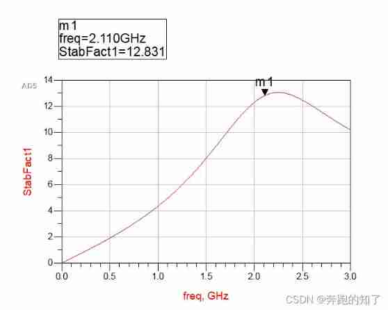
ADS simulation design of class AB RF power amplifier

03 FastJson 解决循环引用

Interruption system of 51 single chip microcomputer
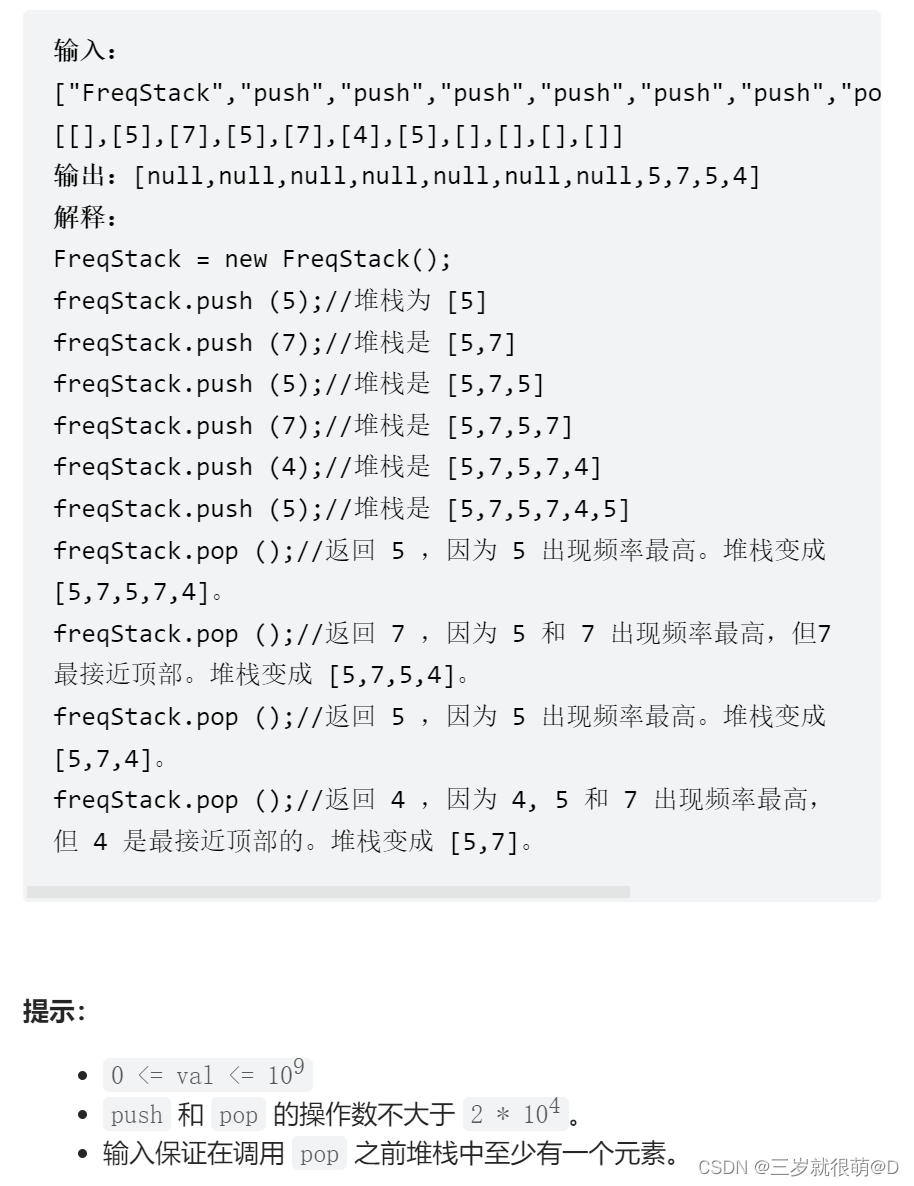
LeetCode - 895 最大频率栈(设计- 哈希表+优先队列 哈希表 + 栈) *

Yocto Technology Sharing Phase 4: Custom add package support
SCM career development: those who can continue to do it have become great people. If they can't endure it, they will resign or change their careers

LeetCode - 703 数据流中的第 K 大元素(设计 - 优先队列)
yocto 技術分享第四期:自定義增加軟件包支持
03 fastjason solves circular references
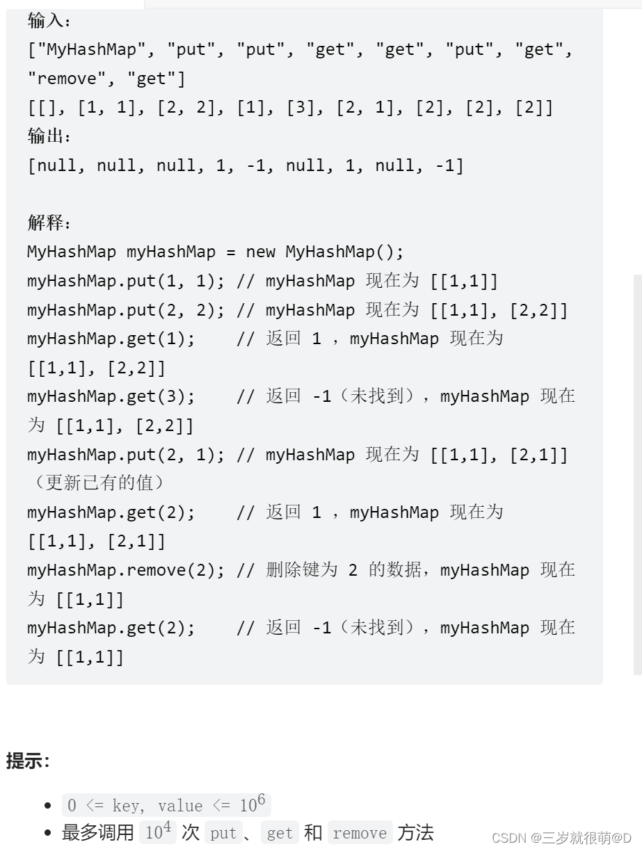
LeetCode - 706 设计哈希映射(设计) *
随机推荐
Blue Bridge Cup for migrant workers majoring in electronic information engineering
LeetCode - 673. 最长递增子序列的个数
After clicking the Save button, you can only click it once
03 FastJson 解决循环引用
Notes on C language learning of migrant workers majoring in electronic information engineering
Pycharm cannot import custom package
On the problem of reference assignment to reference
Uniapp realizes global sharing of wechat applet and custom sharing button style
(1) What is a lambda expression
03 fastjason solves circular references
Screen display of charging pile design -- led driver ta6932
2020-08-23
Serial communication based on 51 single chip microcomputer
Qcombox style settings
is_ power_ of_ 2 judge whether it is a multiple of 2
For new students, if you have no contact with single-chip microcomputer, it is recommended to get started with 51 single-chip microcomputer
Octave instructions
Seven sorting of ten thousand words by hand (code + dynamic diagram demonstration)
自动装箱与拆箱了解吗?原理是什么?
STM32 general timer 1s delay to realize LED flashing