When we're learning and copying garbage collection (Garbage Collection, Abbreviation for GC) Related algorithms and source code , The inner details are inseparable from
These two categories of search algorithms support . That's the context of the build *, The orientation of the article is to eliminate illiteracy through science popularization .
0. Quotation and table of contents
[0] You know - node or node ? [ Into Science ]
[1] Wikipedia - Breadth first search [ Conceptual reference ]
[2] Wikipedia - Depth-first search [ Conceptual reference ]
[3] Wikipedia - Tree traversal [ Conceptual reference ]
[4] CSDN - Depth first traversal and breadth first traversal of binary tree [ Piracy map ]
[5] Blog Garden - The basic concept of graph of data structure [ Recursive plagiarism ]
[6] Blog Garden - Graph traversal Depth first search and breadth first search [ Deep plagiarism ]
[7] github - Depth search and breadth search [ Presentation material ]
Catalog
1. The concept is introduced
2. Tree example
2.1 The former sequence traversal
2.2 In the sequence traversal
2.3 After the sequence traversal
2.4 Level traversal
2.5 Search algorithm source code
3. Examples of Graphs
3.0 The basic concept of graph
3.0.1 Definition of graph
3.0.2 The basic concept of graph
3.0.3 The two most basic storage structures of graphs
3.0.3.1 Adjacency matrix representation
3.0.3.2 Adjacency table representation
3.1 Depth first search text introduction
3.1.1 Depth first search Introduction
3.1.2 Depth first search graph
3.1.2.1 Depth first search of undirected graph
3.1.2.2 Depth first search of digraphs
3.2 Breadth first search text introduction
3.2.1 Introduction to breadth first search
3.2.2 Breadth first search diagram
3.2.2.1 Breadth first search for undirected graphs
3.2.2.2 Breadth first search of digraph
3.3 Search algorithm source code
3.3.1 An undirected graph represented by an adjacency matrix graph (Matrix Undirected Graph)
3.3.2 A directed graph represented by an adjacency matrix graph (Matrix Directed Graph)
3.3.3 An undirected graph represented by an adjacency linked list graph (List Undirected Graph)
3.3.4 Directed graph represented by adjacency linked list graph (List Directed Graph)
1. The concept is introduced
There are many kinds of traversal algorithms , Here's the most versatile , Depth first traversal and breadth first traversal are two kinds of search algorithms
Explain ( The author's ability is limited ). The basics are sometimes fun , Really? ! ok, Then we go on.
Depth first search algorithm (Depth-First-Search, Abbreviation for DFS), An algorithm for traversing or searching trees or graphs . This algorithm
Will search the branches of the tree as deep as possible . When the node v All sides of have been explored , The search will go back to the discovery node v The starting knot on the side of
spot . This process continues until all nodes accessible from the source node have been found . If there is still an undetected node , Choose one of them
individual As the source node and repeat the above process , The whole process repeats until all nodes are accessed .
Breadth first search algorithm (Breadth-First Search, Abbreviation for BFS), Another translation Width first search , or Search horizontally first , It's a kind of
chart Shape search algorithm . To put it simply , BFS It starts at the root , Traverse the nodes of the tree along the width of the tree . If all nodes are accessed , Then algorithm
in stop .
In Computer Science , Tree traversal ( Also known as Tree search ) It is a kind of graph traversal , According to certain rules , To visit without repetition
The process of planting all the nodes of a tree . The specific access operation may be to check the value of the node , Update node values, etc . Different ways to traverse , Conclusion
The order of points is different . Next, we classify the breadth first and depth first traversal algorithms of binary trees , But they also apply to other tree knots
structure .
Depth-first traversal ( Search for )
The former sequence traversal (Pre-Order Traversal)

Depth-first search - The former sequence traversal : F -> B -> A -> D -> C -> E -> G -> I ->H
In the sequence traversal (In-Order Traversal)

Depth-first search - In the sequence traversal : A -> B -> C -> D -> E -> F -> G -> H -> I
After the sequence traversal (Post-Order Traversal)

Depth-first search - After the sequence traversal : A -> C -> E -> D -> B -> H -> I -> G -> F
Breadth first traversal ( Search for )
Level traversal (Level Order Traversal)

Breadth first search - Level traversal :F -> B -> G -> A -> D -> I -> C -> E -> H
The process of planting all the nodes of a tree . The specific access operation may be to check the value of the node , Update node values, etc . Different ways to traverse , Conclusion
By reading and thinking about the excerpts provided in Wikipedia above , We have a little intuitive cognition about two kinds of traversal algorithms . I don't know if
Some people have such doubts , Why is the name of breadth first search not breadth first search? This name is widely spread , It's better to understand in tree structure
There are more ? At first glance, it does , But don't forget that tree structure is a special graph structure , The complex graph structure may not be intuitive from top to bottom , From left to
On the right, this intuitive feeling . Therefore, width first search terms are not accurate enough in generalization . Ha ha ha . Another cognition is about necessity
Conditions of the . For example, depth and breadth first search contains many different traversal related algorithms , It's not just the ones introduced in the article , This is everybody
We should fully understand it .
2. Tree example

Look at the picture , In the prompt, we can find that the definition of traversal is defined around the access time of the root node ( There are hidden rules , Default left child first
Right sub tree behind the tree ). Next, we express the idea of traversal through specific code . First, we construct a tree structure
/**
 *  Easy to test and describe algorithms ,  use  int node  structure
 */
typedef int node_t;

static void node_printf(node_t value) {
    printf(" %2d", value);
}


struct tree {
    struct tree * left;
    struct tree * right;

    node_t node;
};

static inline struct tree * tree_new(node_t value) {
    struct tree * node = malloc(sizeof (struct tree));
    node->left = node->right = NULL;
    node->node = value;
    return node;
}

static void tree_delete_partial(struct tree * node) {
    if (node->left) tree_delete_partial(node->left);
    if (node->right) tree_delete_partial(node->right);
    free(node);
}

void
tree_delete(struct tree * root) {
    if (root) tree_delete_partial(root);
}
2.1 The former sequence traversal
static void tree_preorder_partial(struct stack * s) {
    struct tree * top;

    // 2.1  Access the top node of the stack ,  And put it out of the stack
    while ((top = stack_pop_top(s))) {
        // 2.2  Do business processing
        node_printf(top->node);

        // 3.  If the root node has a right child ,  Put the right child in the stack
        if (top->right)
            stack_push(s, top->right);
        // 4.  If the root node has left children ,  Put the left child in the stack
        if (top->left)
            stack_push(s, top->left);
    }
}

/*
 *  The former sequence traversal :
 *       Root node  ->  The left subtree  ->  Right subtree
 *
 *  inorder traversal :
 *      1.  First put the root node on the stack
        2.  Access the top node of the stack ,  Do business processing ,  And put it out of the stack
        3.  If the root node has a right child ,  Put the right child in the stack
        4.  If the root node has left children ,  Put the left child in the stack
         repeat  2 - 4  Until the stack is empty
 */
void
tree_preorder(struct tree * root) {
    if (!root) return;

    struct stack s[1];
    stack_init(s);

    // 1.  First put the root node on the stack
    stack_push(s, root);
    //  repeat  2 - 4  Until the stack is empty
    tree_preorder_partial(s);

    stack_free(s);
}
2.2 In the sequence traversal
/*
 *  In the sequence traversal :
 *       The left subtree  ->  Root node  ->  Right subtree
 *
 *  inorder traversal :
 *      1.  First put the root node on the stack
        2.  Put all left children of the current node into the stack ,  Until the left child is empty
        3.  Pop up and access the top elements of the stack ,  Do business processing .
        4.  If there is a right child at the top of the stack ,  Repeat the first  2 - 3 Step ,  Until the stack is empty and there is no node to be accessed
 */
void
tree_inorder(struct tree * root) {
    if (!root) return;

    struct stack s[1];
    stack_init(s);

    tree_inorder_partial(root, s);

    stack_free(s);
}

static void tree_postorder_partial(struct stack * s) {
    struct tree * top;
    //  Record the last stack node
    struct tree * last = NULL;

    //  repeat  1-2  Until the stack is empty
    while ((top = stack_top(s))) {
        // 2.2  If we find that its left and right child nodes are empty ,  You can do business processing ;
        // 2.3  perhaps , If it is found that the previous stack node is its left node or right child node , You can do business processing ;
        if ((!top->left && !top->right) || (last && (last == top->left || last == top->right))) {
            //  Do business processing
            node_printf(top->node);
            //  Out of the stack
            stack_pop(s);
            //  Record this stack node
            last = top;
         } else {
            // 2.4.  otherwise , Indicates that the node is a new node , You need to try to stack its right and left child nodes in turn .
            if (top->right)
                stack_push(s, top->right);
            if (top->left)
                stack_push(s, top->left);
         }
    }
}
2.3 After the sequence traversal
static void tree_postorder_partial(struct stack * s) {
    struct tree * top;
    //  Record the last stack node
    struct tree * last = NULL;

    //  repeat  1-2  Until the stack is empty
    while ((top = stack_top(s))) {
        // 2.2  If we find that its left and right child nodes are empty ,  You can do business processing ;
        // 2.3  perhaps , If it is found that the previous stack node is its left node or right child node , You can do business processing ;
        if ((!top->left && !top->right) || (last && (last == top->left || last == top->right))) {
            //  Do business processing
            node_printf(top->node);
            //  Out of the stack
            stack_pop(s);
            //  Record this stack node
            last = top;
         } else {
            // 2.4.  otherwise , Indicates that the node is a new node , You need to try to stack its right and left child nodes in turn .
            if (top->right)
                stack_push(s, top->right);
            if (top->left)
                stack_push(s, top->left);
         }
    }
}

/*
 *  After the sequence traversal :
 *       The left subtree  ->  Right subtree  ->  Root node
 *
 *  inorder traversal :
 *      1.  Get a node ,  First put it on the stack ,  It must be at the bottom of the stack ,  Later
        2.  At the time of putting out the stack, judge whether there is only left node or right node, or both or none of them .
            If we find that its left and right child nodes are empty ,  You can do business processing ;
            perhaps , If it is found that the previous stack node is its left node or right child node , You can do business processing ;
            otherwise , Indicates that the node is a new node , You need to try to stack its right and left child nodes in turn .
         repeat  1-2  Until the stack is empty
 */
void
tree_postorder(struct tree * root) {
    if (!root) return;

    struct stack s[1];
    stack_init(s);

    // 1.  First put the root node on the stack
    stack_push(s, root);
    //  repeat  1 - 4  Until the stack is empty
    tree_postorder_partial(s);

    stack_free(s);
}
Think about the three ways of depth first search above , The image of the amount of stack space occupied is The former sequence traversal < In the sequence traversal < After the sequence traversal ( Existential
example ). Probably , This is why preorder traversal is the most popular tree depth first search algorithm . For the post order tree traversal code implementation , There are also good versions
How many? . Some are easy to write , It's very fancy and clever , This is a regular engineering version .
2.4 Level traversal
/*
 *  Level traversal :
 *       Root node  ->  The next layer  |  Left node  ->  Right node
 *
 *  inorder traversal :
 *      1.  For nodes that are not empty ,  First add the node to the queue
 *      2.  Pop nodes from the team ,  And do business processing ,  Try to push the left node and the right node into the queue
 *       repeat  1 - 2  The guidance queue is empty
 */
void
tree_level(struct tree * root) {
    if (!root) return;

    q_t q;
    q_init(q);

    // 1.  For nodes that are not empty ,  First add the node to the queue
    q_push(q, root);
    do {
        // 2.1  Pop nodes from the team ,  And do business processing
        struct tree * node = q_pop(q);

        node_printf(node->node);

        // 2.2  Try to push the left node and the right node into the queue
        if (node->left)
            q_push(q, node->left);
        if (node->right)
            q_push(q, node->right);

    //  repeat  1 - 2  The guidance queue is empty
    } while (q_exist(q));

    q_free(q);
}
2.5 Search algorithm source code
3. Examples of Graphs
This chapter will give a brief introduction to depth first search and breadth first search of graphs , And then give C Source code implementation .
3.0 The basic concept of graph
3.0.1 Definition of graph
Definition : chart (Graph) It is composed of the finite non empty set of vertices and the set of edges between vertices , Usually expressed as : G(V, E), among , G Express One Map ,
V yes chart G The set of vertices in , E yes chart G in Set of edges .
What should be noted in the diagram is :
(1) In linear tables we call data elements elements elements , Data elements in the tree are called nodes , Data elements in the diagram , We call it the summit (Vertex).
(2) A linear table can have no elements , Known as the empty table ; There can be no nodes in the tree , It's called the empty tree ; however , No vertex is allowed in a graph ( There is poverty and non emptiness ).
(3) The elements in the linear table are linear , The elements in the tree are hierarchical , and , The relationship between vertices in a graph is represented by edges ( Edge sets can be
empty ).
3.0.2 The basic concept of graph
(1) Undirected graph

If the edge between any two vertices in the graph is undirected ( In short, there is no direction of the edge ), The graph is called undirected graph (Undirected
graphs).
(2) Directed graph

If the edge between any two vertices in the graph is a directed edge ( In short, it's the directional side ), It is called a directed graph (Directed graphs).
(3) Complete graph
① Undirected complete graph : In the undirected graph , If there is an edge between any two vertices , The graph is called undirected complete graph . ( contain n The undirected end of a vertex
There are (n×(n-1))/2 side ) As shown in the figure below :

② Directed complete graph : In a directed graph , If there are two arcs with opposite directions between any two vertices , It is called directed complete graph . ( contain
Yes n The directed complete graph of vertices has n×(n-1) side ) As shown in the figure below :

PS: When a graph approaches a complete graph , It is called dense graph (Dense Graph), And when a graph has fewer edges , It is called a sparse graph (
Spare Graph).
(4) The degree of the vertex
The vertices V Degree (Degree) It refers to the relation between in the figure and V Number of sides associated . For digraphs , Have a good attitude (In-degree) And out
(Out-degree) Points , The degree of a vertex in a digraph is equal to the sum of the in and out degrees of the vertex .
(5) Adjacency
① If two vertices in an undirected graph V and W There is an edge (V, W), It's called the summit V and W Adjacency (Adjacent);
② If there is an edge in a digraph <V, W>, said The vertices V Adjacency to The vertices W , live The vertices W Adjacency from The vertices V;
With (2) Directed graph give an example , Yes <A, D> <B, A> <B, C> <C, A> Adjacency relations .
(6) The head and tail of the arc
In the directed graph , The vertex at the end of the arrow Usually called " Starting point " or " Arctail ", The top of the arrow line go by the name of " terminal point " or " Arc head ". <A, D>
Adjacency , The vertices A It's the tail of the arc , The vertices D It's the arc head .
PS: The edges in an undirected graph use parentheses "()" Express , The edges in a digraph use angle brackets "<>" Express .
(7) route
In the undirected graph , If from the top V The starting point has a set of edges to reach the top W, It's called the summit V To the top W The sequence of vertices of , From vertex V To the top W Of
route (Path).
(8) connected
If from V To W There's a path , It's called the summit V And vertex W It's connected (Connected) Of .
(9) power

Some graphs have edges or arcs with numbers associated with them , The number related to the edge or arc of a graph is called weight (Weight).
Some graphs have edges or arcs with numbers associated with them , The number related to the edge or arc of a graph is called weight (Weight).
3.0.3 The two most basic storage structures of graphs
The storage structure of a graph is to store the information of each vertex in the graph , It also stores the relationship between vertices , therefore , The knot of graph
The structure is more complicated . The storage structures of the two most basic types of graphs are adjacency matrix and adjacency table .
3.0.3.1 Adjacency matrix representation
Of Graphs Adjacency matrix (Adjacency Matrix) The storage mode is Use two arrays to represent the graph . A one-dimensional array stores vertex information in a graph , One
Two dimensional array ( It's called adjacency matrix ) Stores information about the edges or arcs in a graph .
(1) Undirected graph
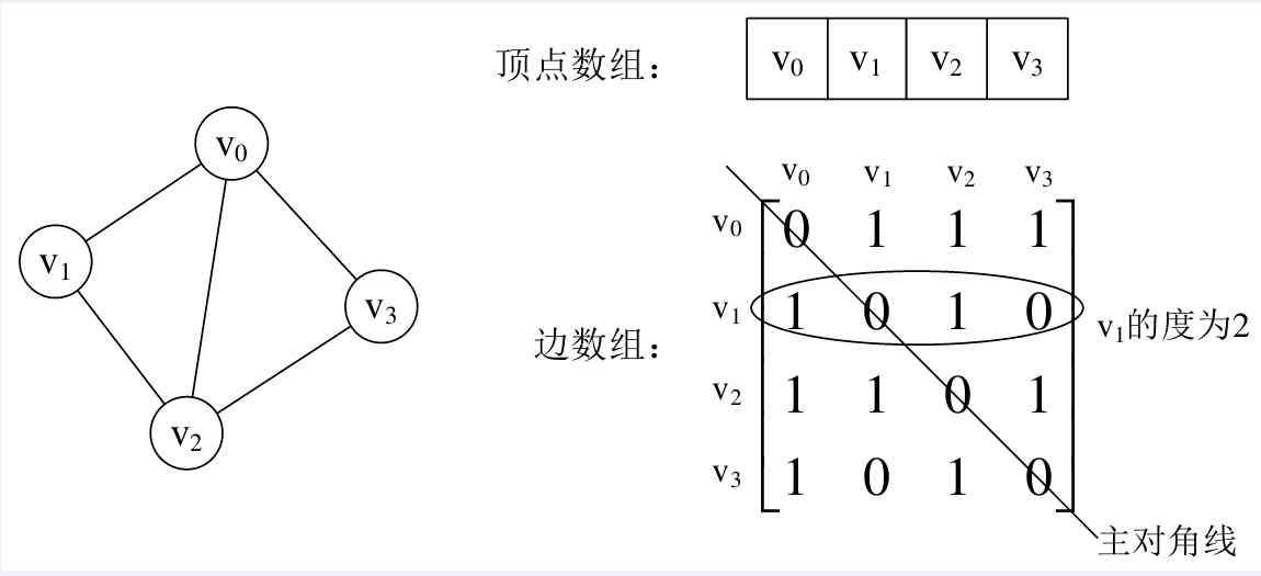
We can set up two arrays , The vertex array is vertex[4] = {V0, V1, V2, V3}, Edge array edges[4][4] This is a moment on the right side of the picture
front . For the value of the principal diagonal of a matrix , namely edges[0][0], edges[1][1], edges[2][2], edges[3][3], All for 0, Because there is no Vertex
Go to your own side .
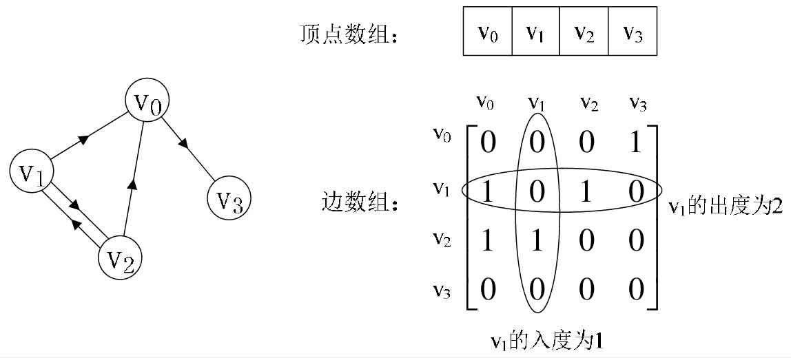
(2) Directed graph
Let's take another example of a digraph , On the left as shown in the figure below . The vertex array is vertex[4] = {V0, V1, V2, V3}, Arc array edges[4][4]
This is a matrix on the right side of the figure below . The value on the main diagonal is still 0. But because it is Directed graph , So this The matrix is not asymmetric , For example, by V1 To V0
Have an arc , obtain edges[1][0] = 1, and V0 To V1 There is no arc , therefore edges[0][1] = 0.
Insufficient : Due to the existence n A graph of vertices needs n*n Array elements to store , When the graph is sparse , Using adjacency matrix storage method will produce
present A lot of 0 Elements , It's a huge waste of space . At this time , Consider using adjacency table representation to store data in a graph .
3.0.3.2 Adjacency table representation
First , Recall the linear table storage structure that we imprinted in our bodies , Sequential storage structure may cause storage space due to the existence of pre allocated memory
The problem of waste , So I think of the chain storage structure . alike , We can also try to use chain storage for edges or arcs to avoid space waves
The question of fee .
Adjacency table by Header node and Tables node Two parts , Each vertex in the graph corresponds to a header node stored in the array . If this watch
The vertex corresponding to the head node has adjacent nodes , Then the adjacent nodes are stored in the one-way linked list pointed to by the header node .
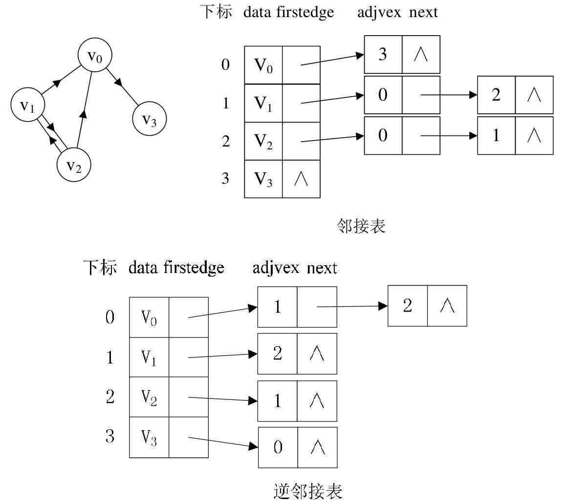
(1) Undirected graph : The graph below shows the adjacency table structure of an undirected graph .
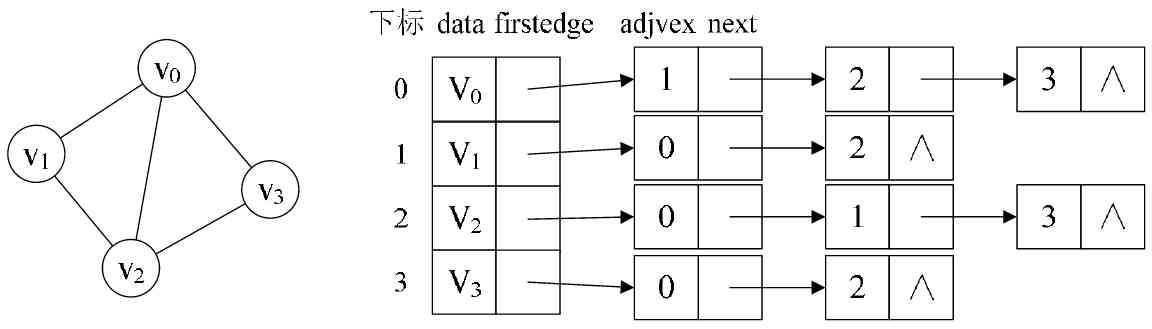
From the picture above, we know that , The nodes of the vertex table are determined by data and firstedge Two fields represent , data It's the data domain , Store vertex information ,
firstedge It's a pointer field , Point to the first node of the edge table , The first adjacent node of this vertex . Edge table nodes are defined by adjvex and next Two domains make up .
adjvex It's a neighborhood , Store the subscript of the adjacency point of a vertex in the vertex table , next Store the pointer to the next node in the edge table . for example :
V1 Vertex and V0, V2 They are adjacency points to each other , It's in V1 In the side table of ,adjvex Respectively V0 Of 0 and V2 Of 2.
PS: For undirected graphs , The use of adjacency list for storage will also lead to data redundancy . For example, in the figure above , The vertices V0 There is... In the linked list
At a pointing vertex V3 At the same time , The vertices V3 There will also be a point in the linked list V0 The summit of .
(2) Directed graph : If there is a digraph , Adjacency table structure is similar , But it should be noted that digraphs have direction . therefore , The adjacency table of a digraph is divided into
Out side table and in side table ( Also called inverse adjacency list ), The table node of the out side table stores the tail node referred to by the directed edge starting from the header node ; The table in the side table
The node stores a vertex that points to the header node , As shown in the figure below .
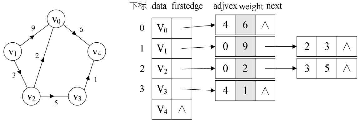
(3) With weight chart : For weighted Net diagram , You can add another... To the definition of the edge table node weight The data field of , Just store the weight information , as follows
As shown in the figure .
3.1 Depth first search text introduction
3.1.1 Depth first search Introduction
Depth first search (Depth First Search), Let's repeat it to deepen our understanding . Let's introduce its search steps : Let's assume that the initial
The state is that all vertices in the graph are not accessed , From some The vertices ( node ) v set out , Access the vertex first , And then, in turn, from each of its not visited
Starting from the adjacent points, depth first search traversal graph , All the way to the sum The vertices v All vertices with paths in common are accessed . If at this time , There are others
The dot was not accessed , Then select another vertex that is not accessed as the starting point , Repeat the process , Until all vertices in the graph are accessed . obviously ,
Depth first search is very easy to construct by recursive process for structures like graphs .
3.1.2 Depth first search graph
3.1.2.1 Depth first search of undirected graph
Let's say " Undirected graph " For example , To demonstrate depth first search .

Right up there chart G1 Conduct depth-first traversal , from The vertices A Start .
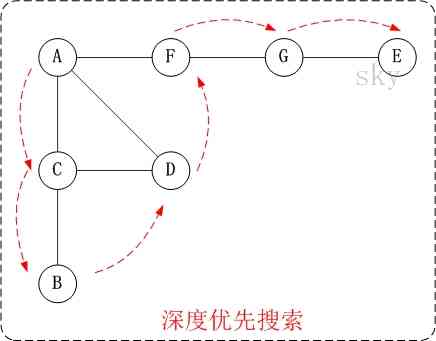
The first 1 Step : visit A.
The first 2 Step : visit (A The adjacency point ) C.
stay The first 1 Step visit A after , What we should visit next is A The adjacency point , namely "C, D, F" One of them . But in the implementation of this paper ,
The vertices ABCDEFG Is stored in order ,C stay "D and F" In front of , therefore , First visit C.
The first 3 Step : visit (C The adjacency point ) B.
stay The first 2 Step visit C after , You should visit C The adjacency point , namely "B and D" In a (A Has been visited , Not included )
. And because the B stay D Before , First visit B.
The first 4 Step : visit (C The adjacency point ) D.
stay The first 3 Step Visited C The adjacency point B after , B There are no adjacent points that are not accessed ; therefore , Return to visit C Another adjacent point of D.
The first 5 Step : visit (A The adjacency point ) F.
I've already visited A, And the interview is over "A The adjacency point B All the adjacency points of ( Including recursive adjacency points )"; therefore , here
Return to visit A Another adjacent point of F.
The first 6 Step : visit (F The adjacency point ) G.
The first 7 Step : visit (G The adjacency point ) E.
So the order of access is : A -> C -> B -> D -> F -> G -> E
3.1.2.2 Depth first search of digraphs
Let's say " Directed graph " For example , To demonstrate depth first search .
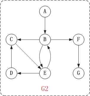
Right up there chart G2 Conduct depth-first traversal , from The vertices A Start .

The first 1 Step : visit A.
The first 2 Step : visit B.
During a visit to the A after , What we should visit next is A The other vertex of the edge of , Vertex B.
The first 3 Step : visit C.
During a visit to the B after , What we should visit next is B The other vertex of the edge of , namely The vertices C, E, F. In the diagram implemented in this paper , The top
spot ABCDEFG Store in order , So first visit C.
The first 4 Step : visit E.
Next visit C The other vertex of the edge of , Vertex E.
The first 5 Step : visit D.
Next visit E The other vertex of the edge of , namely The vertices B, D. The vertices B Has been visited , Therefore access The vertices D.
The first 6 Step : visit F.
Next, we should go back " visit A The other vertex of the edge of F".
The first 7 Step : visit G.
So the order of access is : A -> B -> C -> E -> D -> F -> G
3.2 Breadth first search text introduction
3.2.1 Introduction to breadth first search
Breadth first search algorithm (Breadth First Search), Also known as " Width first search " or " Search horizontally first ", abbreviation BFS. Its traversal
The general idea is : From some vertex in the picture ( node ) v set out , During a visit to the v And then access v Each of the never visited adjacency points , Then separately from
These adjacency points start to visit their adjacency points in turn , And make " The adjacency point of the first visited vertex is accessed before the adjacency point of the later visited vertex
, Until the adjacent points of all the vertices in the graph that have been accessed are accessed . If there are still vertices in the graph that are not accessed , You need to choose another one that hasn't been
Visited vertices as new starting points , Repeat the process , Until all vertices in the graph are accessed . let me put it another way , Breadth first search traversal
The process of graph is to v As a starting point , From near to far , Visit and v There are paths connected and ' The length of the path ' by 1, 2 ... The summit of .
3.2.2 Breadth first search diagram
3.2.2.1 Breadth first search for undirected graphs
Let's say " Undirected graph " For example , To demonstrate breadth first search . Or on top chart G1 Take an example to illustrate .

The first 1 Step : visit A.
The first 2 Step : Sequential access C, D, F.
During a visit to the A after , Next visit A The adjacency point . I've said that before , In the implementation of this paper , The vertices ABCDEFG Store in order
Of , C stay "D and F" In front of , therefore , First visit C. End of visit C after , And then visit D, F.
The first 3 Step : Sequential access B, G.
stay The first 2 Step End of interview C, D, F after , Then visit their neighbors in turn . First visit C The adjacency point B, Revisit F The adjacency point G.
The first 4 Step : visit E.
stay The first 3 Step End of interview B, G after , Then visit their neighbors in turn . Only G There are neighbors E, Therefore access G The adjacency point E.
So the order of access is : A -> C -> D -> F -> B -> G -> E
3.2.2.2 Breadth first search of digraph
Let's say " Directed graph " For example , To demonstrate breadth first search . Or on top chart G2 Take an example to illustrate .

The first 1 Step : visit A.
The first 2 Step : visit B.
The first 3 Step : Sequential access C, E, F.
During a visit to the B after , Next visit B The other vertex of the edge of , namely C, E, F. I've said that before , In the implementation of this paper , The vertices
ABCDEFG Stored in order , So we will visit C, And then visit E, F.
The first 4 Step : Sequential access D, G.
After the interview C, E, F after , Then visit the other vertex of their edge in turn . Or in accordance with C, E, F Sequential access to , C It's all
I visited , Then there's only... Left E, F; First visit E The adjacency point D, Revisit F The adjacency point G.
So the order of access is :A -> B -> C -> E -> F -> D -> G