当前位置:网站首页>Lightgbm principle and its application in astronomical data
Lightgbm principle and its application in astronomical data
2022-07-02 21:56:00 【yellow】

1 LightGBM brief introduction
Light gradient boosting machine(LightGBM) Is a sampling with unilateral gradient (gradient-based one-side sampling,GOSS) Bundled with mutually exclusive features (exclusive feature bundling,EFB) Gradient lifting decision tree (gradient boosting decision tree,GBDT). LightGBM Use histogram method (histogram-based algorithm) Find the best split node of each tree , So the speed is faster than traditional GBDT faster . LightGBM Use GOSS Exclude samples with small residuals in each tree , And focus on large residual samples ( Reduce sample size , Improve model generalization ability );LightGBM Use EFB Focus on samples with large feature dimensions , Reduce the influence of sparse features ( Be similar to PCA Dimension reduction ).
2 LightGBM principle
LightGBM It is a gradient lifting decision tree model with unilateral gradient sampling and mutually exclusive features , Each decision tree uses histogram method to find the best split node .
The following description only considers large sample regression prediction , And it does not describe the binding of mutually exclusive features ( Because feature engineering is often better than mutually exclusive feature bundling , Use LightGBM When processing features , Try to use other methods ; On the other hand, the characteristic dimension of astronomical photometry data used by the author is only 6, Mutually exclusive feature bundling does not work , When using spectral data later , Then we will study the principle of complementary mutually exclusive feature binding )!
2.1 Gradient lift decision tree (GBDT)
In machine learning , If the performance of a model is slightly better than random guess , Then the model can be called weak learner .GBDT It is a class that uses regression decision tree as weak learner Boosting Integrated model , That is to build multiple regression decision trees in series , The final regression prediction is the sum of all decision trees ( It can also be weighted and summed ). This section details GBDT principle , Partial content reference Friedman(2001).
If by Sample sets , among For the first time A sample of Characteristic dimensions , by The response value of . Input ,GBDT The output value is :
among by GBDT The number of regression decision trees in , It's No A regression decision tree , For the first time A regression decision tree about The predicted value of .GBDT Use the following 4 Step by step :
1. initialization . 2. Calculate the residuals , Get the sample set :
3. Fitting sample set O Get the regression decision tree . 4. to update .
The integration model is often in the above section 3 Step uses different ways to fit .GBDT Use the simplest way to fit the decision tree , namely , Sample set O It is recursively divided into two regions by the parent node ( Left 、 Right child node ). Every area ( Left 、 Right child node ) By executing the following 3 Step build a binary decision tree to determine :
1. Start at the root node , Choose the best partition variable And the optimal segmentation point ( Variable The value of ), And minimize the predicted and actual values of the two regions ( Left 、 The right child node ) The mean square error of :
among
And Left 、 The predicted value of the right node .
2. In the 1 After step , Use left 、 The right child node is the new parent node for the next split . According to section 1 Step , Split the new parent node . 3. Repeat the first 1 Step and step 2 Step establishment Establishment and completion !
After the above 3 Step after , Establishment and completion ! However , aggregate The residuals in are different , Small residuals mean GBDT The predicted value almost converges to the real value , Fitting small residual samples again will increase the risk of model over fitting , And build Time consuming . In order to overcome these problems , Unilateral gradient sampling and histogram method are added to GBDT, This is also LightGBM The advantages of the model .
2.2 One side gradient sampling (GOSS)
Unilateral gradient sampling is a way to treat data sets differently Statistical methods for different residuals in . This method eliminates data sets randomly Small and medium residual samples , That is change GBDT The first 2 Step The medium sample size improves the generalization ability of the model . Unilateral gradient sampling is carried out through the following 3 Step implementation :
1. Put the dataset Sort the residuals in , Might as well set :
2. Before the first step The data set corresponding to the residual is recorded as a set ; The data set corresponding to the residual error is recorded as a set , contain Small residual .
among .
3. From the collection Take... At random It's a collection . aggregate Only some small residual samples are included , In order to reduce the impact of data distribution on the model , The collection Multiply the medium residual by the coefficient , namely ,
among .
Above 3 Step corresponds to GBDT The first 2 Step calculate the residual to construct a set ,Ke et al.(2017) Proved that compared with GBDT Model , Unilateral gradient sampling improves the generalization ability of the model by focusing on large sample residuals .
2.2 Histogram method (Histogram-based Algorithm)
It is a time-consuming process to find the best split node by regression decision tree , This is also GBDT The main reason for the slow speed . To alleviate the problem ,Ke et al.(2017) Use histogram method to store continuous variable values in discrete boxes , These boxes are used to construct feature histograms during training . namely , The first A variable In ascending order, it is divided into In a box , Each box contains Samples .
here , Search for the first The best splitting node of variables From the scope Change into . Final , In collection in , Similar to the formula (1), The best splitting node is obtained by the following formula , Then the optimal regression decision tree is constructed .
among
And Left 、 The predicted value of the right node .
Histogram method by reducing GBDT Of the 3 The number of split nodes in the step ( from Down to individual , among Far greater than ) Achieve the effect of acceleration .
3 LightGBM Application
3.1 Related environments and dependent packages
A virtual environment :Python 3.6.2
Related packages :LightGBM 3.2.1 + bayesian-optimization 1.2.0 + pandas 1.1.5 + numpy 1.19.5 + matplotlib 3.3.3 + scikit-learn 0.24.2
Relevant packages are downloaded in pip( perhaps conda) + install + Package name ( Pay attention to the version number ), Such as pip install lightgbm==3.2.1.
3.2 Data set introduction
The experiment purpose : Use Sky Survey photometric data ( the magnitude ) Predict the physical parameters of stellar atmosphere .
The input variable :X, originate SAGE Sky Survey and Pan-STARRS DR1 Cross photometric data (uvgriz,6 A variable ).
Output variables :y, originate APOGEE DR16 Physical parameters of stellar atmosphere ( Effective temperature ,log g Surface gravitational acceleration ,[Fe/H] Abundance of metal ).
Description of data set division :37979 sample size , Press 8:2 Divide training set and test set , In the training set, Bayesian optimization is used for cross validation and parameter adjustment .
3.3 Python Code implementation ( With For example ,log g And [Fe/H] similar )
Transfer Library
# 1.  Data analysis general library
import pandas as pd
import numpy as np
import matplotlib.pyplot as plt
import matplotlib

# 2.  Data set partition Library
from sklearn.model_selection import train_test_split, cross_val_score

# 3.  Data processing 、 Feature construction library
from sklearn.preprocessing import MinMaxScaler
from sklearn.decomposition import PCA

# 4.  Evaluation index database
import sklearn.metrics as sm

# 5.  Model tuning Bayesian Optimization Library
from bayes_opt import BayesianOptimization

# 6.  call LightGBM library
import lightgbm as lgb

# 7.  Visual decision tree Library , Need to download ahead of time Graphviz, Otherwise, just comment it out !
import os
os.environ["PATH"] += os.pathsep + 'D:/Graphviz/bin'

# 8.  Fine tuning of drawing settings
matplotlib.rcParams["font.family"] = "SimHei"
matplotlib.rcParams["axes.unicode_minus"] = False
#  take x、y The direction of the scale line of the shaft is set inward
plt.rcParams['xtick.direction'] = 'in'
plt.rcParams['ytick.direction'] = 'in'
Data reading and feature construction
# 9.  Data set read , Rename column name .
data = pd.read_csv("new_data.csv")
x_data = data[["UMAG", "VMAG", "RMAG", "IMAG", "ZMAG", "GMAG"]]
y_data = data["TEFF"]
x_data.columns = ["u", "v", "r", "i", "z", "g"]
y_data.columns = ["Teff"]

# 10.  Data set partitioning , Set random seeds to make the model reproducible .
x_train, x_test, y_train, y_test = train_test_split(x_data, y_data, train_size=0.8, random_state=1)
# 11.  Normalized independent variable X, The test set is normalized according to the training set .
scaler1 = MinMaxScaler().fit(x_train)
x_train = scaler1.transform(x_train)
x_test = scaler1.transform(x_test)

# 12.  Principal component transformation argument X, The test set is conducted in the way of training set , And rename the name of the column .
pca = PCA(n_components=6, random_state=666).fit(x_train)
x_train = pca.transform(x_train)
x_test = pca.transform(x_test)
x_train = pd.DataFrame(x_train, columns=["F1", "F2", "F3", "F4", "F5", "F6"])
x_test = pd.DataFrame(x_test, columns=["F1", "F2", "F3", "F4", "F5", "F6"])
Bayesian Optimization tuning
# 13.  Design of Bayesian optimization objective function :LGBM_cv(). The variable in the function is LightGBM Model parameters to be adjusted , Use 5 Fold cross validation for Bayesian parameter adjustment !
# top_rate, other_rate Respectively LIghtGBM In the model a And b, That is, the proportion of samples with large residuals and small residuals .
#  Histogram method is mainly to accelerate , This is not used as a super parameter adjustment , Because we value LightGBM The speed of , So take the default 255.
def LGBM_cv(learning_rate, num_leaves, max_depth, subsample, min_child_samples, n_estimators, feature_fraction, feature_fraction_bynode, lambda_l2, top_rate, other_rate
          ):
    val = cross_val_score(lgb.LGBMRegressor(objective='regression_l2',
                            boosting_type="goss",
                            top_rate=top_rate,
                            other_rate=other_rate,
                            random_state=666,
                            learning_rate=learning_rate,
                            num_leaves=int(num_leaves),
                            max_depth=int(max_depth),
                            subsample=subsample,
                            min_child_samples=int(min_child_samples),
                            n_estimators=int(n_estimators),
                            colsample_bytree=feature_fraction,
                            feature_fraction_bynode=feature_fraction_bynode,
                            reg_lambda=lambda_l2,
                            ),
                          X=x_train, y=y_train, verbose=0, cv=5, scoring=sm.make_scorer(sm.mean_squared_error)).mean()
    return -1 * val ** 0.5

# 14.  Setting the domain space in the objective function ( Parameter range , Set it up by yourself , Don't refer to what I wrote ).
LGBM_bo = BayesianOptimization(
    LGBM_cv,
    {
    'learning_rate': (0.03, 0.038),
    'num_leaves': (36, 44),
    'max_depth': (8, 10),
    'subsample': (0.58, 0.64),
    'min_child_samples' : (20, 30),
    'n_estimators': (900, 1000),
    'feature_fraction': (0.9, 0.98),
    'feature_fraction_bynode': (0.83, 0.91),
    'lambda_l2': (0.04, 0.11),
    'top_rate': (0.12, 0.16),
    'other_rate': (0.4, 0.46),
    },
    random_state=666
)

# 15.  Initial value of parameter range , If the parameter value with higher accuracy is known , It can be used as the initial value . It can be used to fine tune parameters !
LGBM_bo.probe(
    params={
        'feature_fraction': 0.9426045698173733,
        'feature_fraction_bynode': 0.8759128982908615,
        'lambda_l2': 0.07262385457770391,
        'learning_rate': 0.034418220958292195,
        'max_depth': 9,
        'min_child_samples': 25,
        'n_estimators': 976,
        'num_leaves': 40,
        'other_rate': 0.42355836143730674,
        'subsample': 0.6095003877871213,
        'top_rate': 0.14308601351231862

    },
    lazy=True,
)

# 16.  Set the number of Bayesian Optimization iterations n_iter, And the number of random attempts after the iteration init_points.
LGBM_bo.maximize(n_iter=200, init_points=20)

# 17.  Output optimal parameter combination , And save the best parameters , Convenient for model training and testing .
print(LGBM_bo.max)
print("target:", LGBM_bo.max["target"])
params = LGBM_bo.max["params"]
feature_fraction = params["feature_fraction"]
feature_fraction_bynode = params["feature_fraction_bynode"]
lambda_l2 = params["lambda_l2"]
learning_rate = params["learning_rate"]
max_depth = int(params["max_depth"])
min_child_samples = int(params["min_child_samples"])
n_estimators = int(params["n_estimators"])
num_leaves = int(params["num_leaves"])
subsample = params["subsample"]
top_rate = params["top_rate"]
other_rate = params["other_rate"]

Use the best parameters for training and prediction
# 18. LightGBM The model uses Bayes to adjust the optimal parameters for training and prediction .
clf = lgb.LGBMRegressor(objective='regression_l2',
random_state=666,
boosting_type="goss",
learning_rate=learning_rate,
max_depth=max_depth,
min_child_samples=min_child_samples,
n_estimators=n_estimators,
num_leaves=num_leaves,
subsample=subsample,
feature_fraction=feature_fraction,
feature_fraction_bynode=feature_fraction_bynode,
lambda_l2=lambda_l2,
top_rate=top_rate,
other_rate=other_rate,
importance_type="gain",
).fit(x_train, y_train)
pred_train = clf.predict(x_train)
pred_test = clf.predict(x_test)
# 19. Calculate the evaluation index , Determinable coefficient , Root mean square error and mean absolute error .
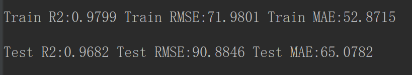
print("Train R2:%.4f" % sm.r2_score(y_train, pred_train))
print("Train RMSE:%.4f" % (sm.mean_squared_error(y_train, pred_train) ** 0.5))
print("Train MAE:%.4f" % (sm.mean_absolute_error(y_train, pred_train)))
print("Test R2:%.4f" % sm.r2_score(y_test, pred_test))
print("Test RMSE:%.4f" % (sm.mean_squared_error(y_test, pred_test) ** 0.5))
print("Test MAE:%.4f" % (sm.mean_absolute_error(y_test, pred_test)))
Visualization of test set prediction results
# 20.  Draw density map using this library .
from scipy.stats import gaussian_kde

pred_test = np.array(pred_test).reshape(-1)
y_test = np.array(y_test).reshape(-1)
xy = np.vstack([pred_test, y_test])
z1 = gaussian_kde(xy)(xy)

pred_test_residual = np.array(y_test - pred_test).reshape(-1)
pred_test = np.array(pred_test).reshape(-1)
xy = np.vstack([pred_test, pred_test_residual])
z2 = gaussian_kde(xy)(xy)

fig = plt.figure(figsize=(10, 8), dpi=300)
gs = fig.add_gridspec(2, 1, hspace=0, wspace=0.2, left=0.13, top=0.98, bottom=0.1)
(ax1), (ax2) = gs.subplots(sharex='col')

ax11 = ax1.scatter(pred_test.tolist(), y_test.tolist(), s=2, c=z1)
ax1.plot([np.min(pred_test)-500, np.max(pred_test)+500], [np.min(pred_test)-500, np.max(pred_test)+500], "--", linewidth=1.5)
ax1.set_ylabel(r"$Test$", fontsize=25)
ax1.xaxis.set_major_locator(plt.MaxNLocator(3))
ax1.yaxis.set_major_locator(plt.MaxNLocator(4))
ax1.tick_params(top='on', right='on', which='both', labelsize=25)
ax1.set_xlim([np.min(pred_test)-500, np.max(pred_test)+500])
ax1.set_ylim([np.min(pred_test)-500, np.max(pred_test)+500])
ax1.xaxis.set_major_locator(plt.MultipleLocator(1000))
ax1.yaxis.set_major_locator(plt.MultipleLocator(1000))
ax1.xaxis.set_minor_locator(plt.MultipleLocator(250))
ax1.yaxis.set_minor_locator(plt.MultipleLocator(250))

ax2.scatter(pred_test.tolist(), (y_test - pred_test).tolist(), s=2, c=z2)
ax2.plot([np.min(pred_train)-500, np.max(pred_train)+500], [0, 0], "--", linewidth=1.5)
ax2.set_title(r"$σT_{eff}=%.i$" % (np.var(y_test - pred_test) ** 0.5), fontsize=25)
ax2.set_xlabel(r"$Pred \ T_{eff}(k)$", fontsize=25)
ax2.set_ylabel(r"$Residual$", fontsize=25)
ax2.tick_params(top='on', right='on', which='both', labelsize=25)
ax2.xaxis.set_major_locator(plt.MultipleLocator(1000))
ax2.yaxis.set_major_locator(plt.MultipleLocator(400))
ax2.xaxis.set_minor_locator(plt.MultipleLocator(250))
ax2.yaxis.set_minor_locator(plt.MultipleLocator(100))

plt.rcParams['font.size'] = 25
fig.colorbar(ax11,
             label="Density",
             cax=fig.add_axes([0.92, 0.1, 0.02, 0.86]), ax=(ax1, ax2))
plt.show()

LightGBM The importance of model features
LightGBM The importance of model features : During the whole fitting process , The ratio of the number of node splits of all variables to the total number of splits of all variables . Feature importance ranking can be further analyzed in combination with astronomical features , Explain the stability of the model .
plt.style.use("ggplot")
plt.figure(dpi=300)
plt.rcParams['font.size'] = 18
importance = pd.DataFrame({"importance": np.round(clf.feature_importances_ / np.sum(clf.feature_importances_), 3),
                          "names": x_train.columns})
importance = importance.sort_values(by="importance", ascending=True)
plt.barh(y=importance["names"],
         width=importance["importance"], height=0.2)
for a, b, label in zip(importance["importance"], importance["names"], importance["names"]):
    plt.text(a+0.06, b, "%.1f" % (a*100) + "%", ha='center', va='center', fontsize=14)
plt.title(r"$T_{eff}$ Feature importance", fontsize=18)
plt.xlabel("Feature importance", fontsize=18)
plt.ylabel("Features", fontsize=18)
plt.xticks(fontsize=16)
plt.yticks(fontsize=20)
plt.xlim([0, 1])
plt.gca().xaxis.set_major_locator(plt.MaxNLocator(4))
plt.show()

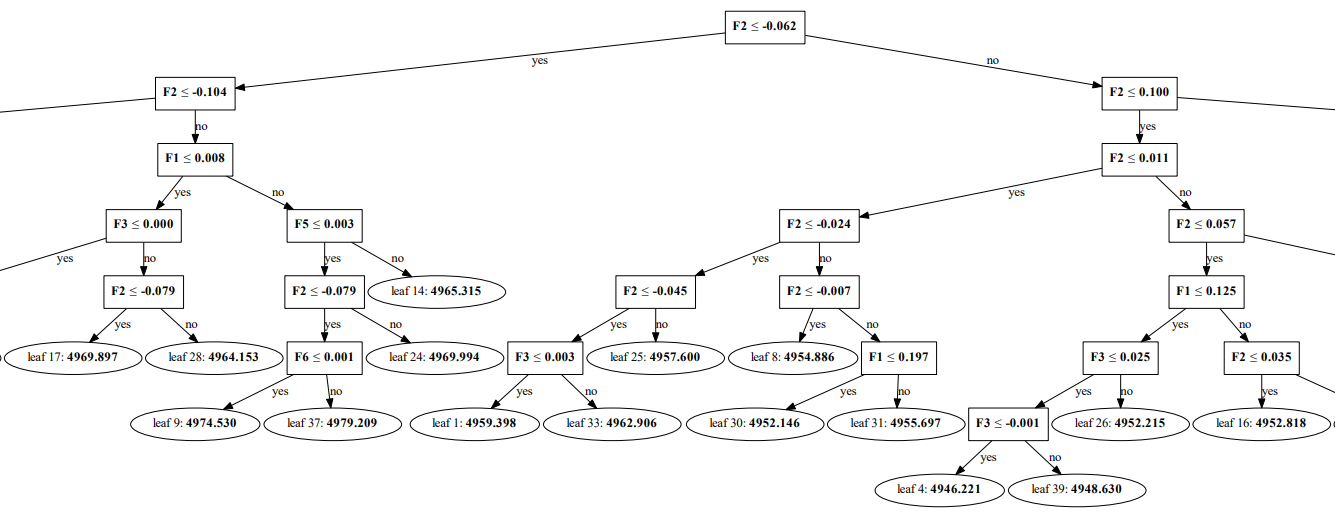
see LightGBM Model any tree
# 21.  Look at the first 1 Tree split pattern .
dot_data = lgb.create_tree_digraph(clf, orientation="vertical", tree_index=0, name="tree1")
dot_data.format = 'PDF'
dot_data.render('TEFF_1.pdf')
LightGBM in GOSS Quantitative analysis of
Range , Other parameters are optimal . The red dots in the figure below , When , when , The error is the lowest .
# 22. 3 Uygur painting gallery .
from mpl_toolkits.mplot3d import Axes3D
from matplotlib import cm

RMSE = []
k = 12
A = np.linspace(0.01, 0.5, k)
B = np.linspace(0.01, 0.5, k)
for i in A:
    for j in B:
        clf = lgb.LGBMRegressor(objective='regression_l2',
                                random_state=666,
                                boosting_type="goss",
                                learning_rate=learning_rate,
                                max_depth=max_depth,
                                min_child_samples=min_child_samples,
                                n_estimators=n_estimators,
                                num_leaves=num_leaves,
                                subsample=subsample,
                                feature_fraction=feature_fraction,
                                lambda_l2=lambda_l2,
                                top_rate=i,
                                other_rate=j,
                                max_bin=max_bin,
                                importance_type="gain",
                                ).fit(x_train, y_train)
        pred_train = clf.predict(x_train)
        pred_test = clf.predict(x_test)

        RMSE.append(sm.mean_squared_error(y_test, pred_test) ** 0.5)
        print(i)
        print("Train R2:%.4f" % sm.r2_score(y_train, pred_train))
        print("Train RMSE:%.4f" % (sm.mean_squared_error(y_train, pred_train) ** 0.5))
        print("Train MAE:%.4f" % (sm.mean_absolute_error(y_train, pred_train)))
        print("Test R2:%.4f" % sm.r2_score(y_test, pred_test))
        print("Test RMSE:%.4f" % (sm.mean_squared_error(y_test, pred_test) ** 0.5))
        print("Test MAE:%.4f" % (sm.mean_absolute_error(y_test, pred_test)))

A, B = np.meshgrid(A, B)
RMSE = np.array(RMSE).reshape(k, k)
min_RMSE = np.argwhere(RMSE == np.min(RMSE))
min_A = A[min_RMSE[0][0], min_RMSE[0][1]]
min_B = B[min_RMSE[0][0], min_RMSE[0][1]]
min_RMSE = RMSE[min_RMSE[0][0], min_RMSE[0][1]]
print(min_A, min_B, min_RMSE)
fig, ax = plt.subplots(subplot_kw=dict(projection='3d'))
surf = ax.plot_surface(A, B, RMSE, cmap=cm.coolwarm, alpha=0.8)
ax.xaxis.set_major_locator(LinearLocator(5))
ax.yaxis.set_major_locator(LinearLocator(5))
ax.zaxis.set_major_locator(LinearLocator(5))
ax.xaxis.set_major_formatter(FormatStrFormatter('%.02f'))
ax.yaxis.set_major_formatter(FormatStrFormatter('%.02f'))
ax.zaxis.set_major_formatter(FormatStrFormatter('%.i'))
ax.set_xlabel(r'$a$', size=15)
ax.set_ylabel(r'$b$', size=15)
ax.set_xlim3d(0.01, 0.5)
ax.set_ylim3d(0.01, 0.5)
ax.set_zlim3d(88, 95)
ax.set_title("Influence of GOSS on Teff prediction RMSE", weight='bold', size=15)
fig.colorbar(surf, shrink=0.6, aspect=8, label="RMSE")
ax.scatter(min_A, min_B, min_RMSE, marker="o", c="r", s=20)
plt.show()

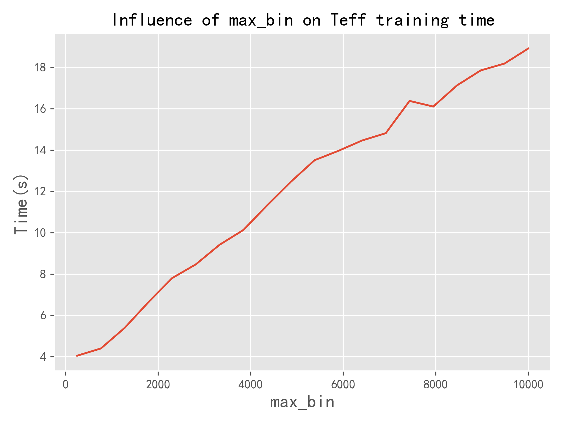
LightGBM Quantitative analysis of histogram method in
Box quantity range (s) by , step , Other parameters are optimal . As shown in the figure below , As the number of boxes increases , Model training time increases linearly . Appropriate s Value , yes LIghtGBM The important reason why the model is faster .
# 23.  Time bank .
import time

RMSE = []
TIME = []
max_bin = np.linspace(250, 10000, 20)
print(max_bin)
for i in max_bin:
    time0 = time.time()
    clf = lgb.LGBMRegressor(objective='regression_l2',
                            random_state=666,
                            boosting_type="goss",
                            learning_rate=learning_rate,
                            max_depth=max_depth,
                            min_child_samples=min_child_samples,
                            n_estimators=n_estimators,
                            num_leaves=num_leaves,
                            subsample=subsample,
                            feature_fraction=feature_fraction,
                            lambda_l2=lambda_l2,
                            top_rate=top_rate,
                            other_rate=other_rate,
                            max_bin=int(i),
                            importance_type="gain",
                            ).fit(x_train, y_train)
    pred_train = clf.predict(x_train)
    pred_test = clf.predict(x_test)
    TIME.append(time.time() - time0)
    RMSE.append(sm.mean_squared_error(y_test, pred_test) ** 0.5)
    print(i)
    print(" Time consuming ", time.time() - time0)
    print("Train R2:%.4f" % sm.r2_score(y_train, pred_train))
    print("Train RMSE:%.4f" % (sm.mean_squared_error(y_train, pred_train) ** 0.5))
    print("Train MAE:%.4f" % (sm.mean_absolute_error(y_train, pred_train)))
    print("Test R2:%.4f" % sm.r2_score(y_test, pred_test))
    print("Test RMSE:%.4f" % (sm.mean_squared_error(y_test, pred_test) ** 0.5))
    print("Test MAE:%.4f" % (sm.mean_absolute_error(y_test, pred_test)))

plt.style.use("ggplot")
plt.figure(dpi=300)
plt.plot(max_bin, TIME)
plt.xlabel("max_bin", fontsize=15)
plt.ylabel("Time(s)", fontsize=15)
plt.title("Influence of max_bin on Teff training time", size=15)
plt.show()
LightGBM VS Some machine learning models
To illustrate LightGBM The high performance of the model , Using the same dataset 、 Bayesian optimization method is compared with random forest 、XGBoost、GBDT、ANN、SVR And the prediction results of linear regression in the test set . You can find ,LightGBM Is a faster model , And the generalization ability is slightly stronger . therefore , It is suitable for data analysis in the era of big data .
summary
Mainly about LightGBM The principle of the model and its application in astronomy , The principle part refers to Ke(2017) And Liang(2022), The astronomical application part is taken from Liang(2022). A detailed analysis of LightGBM Of GOSS And the performance improvement brought by histogram ,GOSS It mainly improves the generalization ability of the model , Histograms are used to speed up . For experimental needs , There is no discussion of mutually exclusive feature bundling (EFB) as well as LightGBM According to the leaf growth strategy , regret !
Please refer to LightGBM: A Highly Efficient Gradient Boosting Decision Tree Guolin[1] And Estimation of Stellar Atmospheric Parameters with Light Gradient Boosting Machine Algorithm and Principal Component Analysis[2]
Reference material
Document address : https://proceedings.neurips.cc/paper/2017/hash/6449f44a102fde848669bdd9eb6b76fa-Abstract.html
[2]Document address : https://iopscience.iop.org/article/10.3847/1538-3881/ac4d97
边栏推荐
- The failure rate is as high as 80%. What should we do about digital transformation?
- 技术人创业:失败不是成功,但反思是
- Find objects you can't see! Nankai & Wuhan University & eth proposed sinet for camouflage target detection, and the code has been open source
- [leetcode] sword finger offer 04 Search in two-dimensional array
- Research Report on plastic antioxidant industry - market status analysis and development prospect forecast
- ~91 rotation
- SQL必需掌握的100个重要知识点:使用游标
- 图像基础概念与YUV/RGB深入理解
- 地理探测器原理介绍
- : last child does not take effect
猜你喜欢
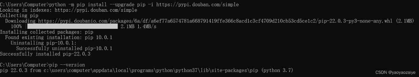
PIP version update timeout - download using domestic image
![[shutter] statefulwidget component (pageview component)](/img/0f/af6edf09fc4f9d757c53c773ce06c8.jpg)
[shutter] statefulwidget component (pageview component)

Daily book -- analyze the pain points of software automation from simple to deep
关于测试用例

腾讯三面:进程写文件过程中,进程崩溃了,文件数据会丢吗?

"New programmer 003" was officially launched, and the cloud native and digital practical experience of 30+ companies such as Huawei and Alibaba
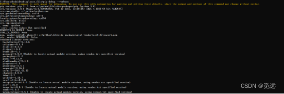
pip安裝whl文件報錯:ERROR: ... is not a supported wheel on this platform
Pip install whl file Error: Error: … Ce n'est pas une roue supportée sur cette plateforme
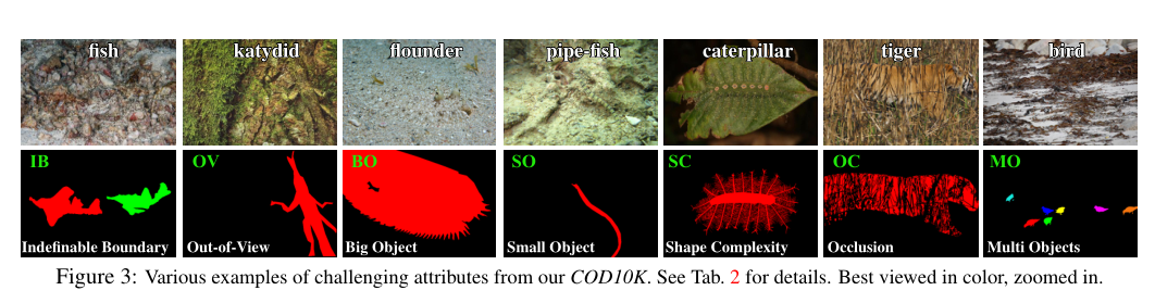
发现你看不到的物体!南开&武大&ETH提出用于伪装目标检测SINet,代码已开源!...

Interpretation of CVPR paper | generation of high fidelity fashion models with weak supervision
随机推荐
Unity3D学习笔记4——创建Mesh高级接口
The failure rate is as high as 80%. What should we do about digital transformation?
加了定位的文字如何水平垂直居中
Oriental Aesthetics and software design
Redis distributed lock failure, I can't help but want to burst
分享一下如何制作专业的手绘电子地图
China microporous membrane filtration market trend report, technological innovation and market forecast
*C language final course design * -- address book management system (complete project + source code + detailed notes)
Official announcement! The golden decade of new programmers and developers was officially released
Free open source web version of xshell [congratulations on a happy new year]
LightGBM原理及天文数据中的应用
How to test the process of restoring backup files?
[shutter] statefulwidget component (pageview component)
攻防世界pwn题:Recho
[shutter] shutter layout component (opacity component | clipprect component | padding component)
TinyMCE visual editor adds Baidu map plug-in
Physical layer cables and equipment
About test cases
LandingSite eBand B1冒烟测试用例
[leetcode] sword finger offer 04 Search in two-dimensional array