Detailed analysis of pytorch's automatic derivation mechanism, pytorch's core magic

Click on the above “ Xiaobai studies vision ”, Optional plus " Star standard " or “ Roof placement ”

 Heavy dry goods , First time delivery 

---

author ：Vaibhav Kumar

compile ：ronghuaiyang

Reading guide

This article analyzes in detail PyTorch Automatic derivation mechanism , Let you know PyTorch Core magic of .

In the process , It never explicitly constructs the entire Jacobian matrix . Direct calculation JVP It's usually simpler 、 More effective .

We all agree that , When it comes to large neural networks , We are not good at calculus . It is unrealistic to calculate the gradient of such a large composite function by explicitly solving mathematical equations , In particular, these curves exist in a large number of dimensions , It's incomprehensible .

To deal with 14 Hyperplane in dimensional space , Imagine a three-dimensional space , Say to yourself loudly “14”. Everyone does this ——Geoffrey Hinton

This is it. PyTorch Of autograd Where it works . It abstracts complex mathematics , Help us “ Miraculously ” Calculate the gradient of high-dimensional curve , Just a few lines of code . This article attempts to describe autograd The magic of .

PyTorch Basics

Before further discussion , We need to know some basic PyTorch Concept .

tensor ： In short , It's just PyTorch One of them n Dimension group . Tensors support some additional enhancements , This makes them unique ： except CPU, They can be loaded or GPU Faster computing . Set up .requires_grad = True When , They began to form a reverse diagram , Tracking is applied to each of their operations , Use the so-called dynamic calculation diagram (DCG) Calculate the gradient ( It will be explained further later ).

In earlier versions PyTorch in , Use torch.autograd.Variable Class is used to create tensors that support gradient computation and operation tracking , But up to PyTorch v0.4.0,Variable Class is disabled .torch.Tensor and torch.autograd.Variable Now it is the same class . More precisely , torch.Tensor Be able to track history and behave like the old Variable.

import torch
 import numpy as np
 
 x = torch.randn(2, 2, requires_grad = True)
 
 # From numpy
 x = np.array([1., 2., 3.]) #Only Tensors of floating point dtype can require gradients
 x = torch.from_numpy(x)
 # Now enable gradient
 x.requires_grad_(True)
 # _ above makes the change in-place (its a common pytorch thing)

Code for creating various methods that enable the tensor of gradients

Be careful ： according to PyTorch The design of the , Gradients can only compute floating-point tensors , This is why I created a floating point type numpy Array , Then set it to gradient enabled PyTorch tensor .

Autograd： This class is an engine for calculating derivatives ( More precisely, Jacobian vector product ). It records a graph of all operations on the gradient tensor , And create an acyclic graph called dynamic calculation graph . The leaf nodes of this graph are input tensors , The root node is the output tensor . The gradient is achieved by tracing the graph from root to leaf , And use the chain rule to multiply each gradient .

Neural networks and back propagation

Neural networks are only carefully tuned ( Training ) A compound mathematical function that outputs the desired result . Adjustment or training is done through an excellent algorithm called back propagation . Back propagation is used to calculate the loss gradient relative to the input weight , So that the weight can be updated later , Ultimately reduce losses .

In a way , Back propagation is just a fancy name for the chain rule —— Jeremy Howard

Creating and training neural networks includes the following basic steps ：

1. Define the architecture

2. Use input data to propagate forward architecturally

3. Calculate the loss

4. Back propagation , Calculate the gradient of each weight

5. Update weights with learning rates

The small change of the input weight caused by the loss change is called the gradient of the weight , And use back propagation to calculate . Then use the gradient to update the weight , Use the learning rate to reduce the loss as a whole and train the neural network .

This is done iteratively . For each iteration , You have to calculate several gradients , And build something called a computational graph for storing these gradient functions .PyTorch By building a dynamic calculation diagram (DCG) To achieve this . This diagram is built from scratch in each iteration , It provides maximum flexibility for gradient calculation . for example , For forward operation ( function )Mul , Backward operation function MulBackward It is dynamically integrated into the backward graph to calculate the gradient .

Dynamic calculation diagram

Tensors that support gradients ( Variable ) And the function ( operation ) Combine to create a dynamic calculation diagram . Data flows and operations applied to data are defined at run time , So as to dynamically construct the calculation diagram . This diagram is composed of the bottom autograd Class dynamically generated . You don't have to code all possible paths before starting training —— What you run is what you distinguish .

A simple DCG The multiplication for two tensors would be like this ：

with requires_grad = False Of DCG

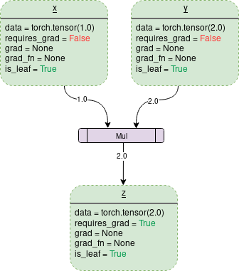
Each point outline box in the figure is a variable , The purple rectangle is an operation .

Each variable object has several members , Some of the members are ：

Data： It is the data held by a variable .x Hold one 1x1 tensor , Its value is equal to 1.0, and y hold 2.0.z Hold the product of two , namely 2.0.

requires_grad： This member ( If true) Start tracking all operation history , And form a backward graph for gradient calculation . For any tensor a, It can be treated in situ as follows ：a.requires_grad_(True).

grad: grad Save the gradient value . If requires_grad by False, It will hold a None value . Even if requires_grad It's true , It will also hold a None value , Unless called from another node .backward() function . for example , If you are right about out About x Calculate the gradient , call out.backward(), be x.grad The value of is ∂out/∂x.

grad_fn： This is the backward function used to calculate the gradient .

is_leaf： If ：

1. It is explicitly initialized by some functions , such as x = torch.tensor(1.0) or x = torch.randn(1, 1)( Basically, all tensor initialization methods discussed at the beginning of this paper ).

2. It is created after the operation of tensor , All tensors have requires_grad = False.

3. It is by calling .detach() Method to create .

Calling backward() when , Only calculate requires_grad and is_leaf At the same time, the gradient of true nodes .

When open requires_grad = True when ,PyTorch The tracking operation will begin , And store the gradient function in each step , As shown below ：

requires_grad = True Of DCG

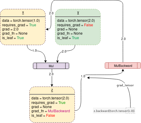
stay PyTorch The code that generates the above figure is ：

Backward() function

Backward Functions actually pass parameters ( By default 1x1 Unit tensor ) To calculate the gradient , It passes through Backward The graph goes all the way to each leaf node , Each leaf node can be traced from the root tensor of the call to the leaf node . Then the calculated gradient is stored in the .grad in . please remember , The backward graph has been dynamically generated in the forward transfer process .backward The function calculates the gradient using only the generated graph , And store it in the leaf node .

Let's analyze the following code ：

import torch
 # Creating the graph
 x = torch.tensor(1.0, requires_grad = True)
 z = x ** 3
 z.backward() #Computes the gradient
 print(x.grad.data) #Prints '3' which is dz/dx

An important thing to pay attention to is , When calling z.backward() when , A tensor is automatically passed as z.backward(torch.tensor(1.0)).torch.tensor(1.0) Is the external gradient used to terminate the chain rule gradient multiplication . This external gradient is passed as input to MulBackward function , To further calculate x Gradient of . Pass on to .backward() The dimension of the tensor in must be the same as that of the tensor in which the gradient is being calculated . for example , If the gradient supports tensor x and y as follows ：

x = torch.tensor([0.0, 2.0, 8.0], requires_grad = True)
 y = torch.tensor([5.0 , 1.0 , 7.0], requires_grad = True)
 z = x * y

then , To calculate z About x perhaps y Gradient of , You need to pass an external gradient to z.backward() function , As shown below ：

z.backward(torch.FloatTensor([1.0, 1.0, 1.0])

z.backward() Will give RuntimeError: grad can be implicitly created only for scalar outputs

The tensor passed by the inverse function is like the weight of the gradient weighted output . Mathematically speaking , This is a vector multiplied by a non scalar tensor Jacobian matrix ( This paper will further discuss ), Therefore, it is almost always a unit tensor of one dimension , And backward Same tensor , Unless you need to calculate the weighted output .

tldr ： The backward graph is composed of autograd Class is automatically and dynamically created during forward passing .Backward() The gradient is calculated simply by passing its parameters to the generated inverse graph . 

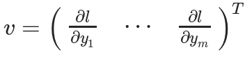
mathematics — Jacobian matrix and vector

Mathematically speaking ,autograd Class is just a Jacobian vector product calculation engine . Jacobian matrix is a very simple word , It represents all possible partial derivatives of two vectors . It's the gradient of one vector relative to another .

Be careful ： In the process ,PyTorch The entire Jacobian matrix is never explicitly constructed . Direct calculation JVP (Jacobian vector product) It's usually simpler 、 More effective .

If a vector X = [x1, x2,…xn] adopt f(X) = [f1, f2,…fn] To calculate other vectors , Then Jacobian matrix (J) Contains all of the following partial derivative combinations ：

Jacobian matrix

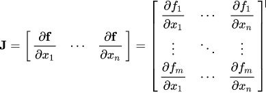
The matrix above represents f(X) be relative to X Gradient of .

Suppose one is enabled PyTorch Tensor of gradient X：

X = [x1,x2,…,xn]( Suppose this is the weight of a machine learning model )

X After some operations, form a vector Y

Y = f(X) = [y1, y2,…,ym]

And then use Y Calculate scalar loss l. Suppose that the vector v It happens to be a scalar loss l About vectors Y Gradient of , as follows ：

vector v be called grad_tensor, And pass it as a parameter to backward() function .

In order to get the gradient of loss l About weight X Gradient of , Jacobian matrix J Is vector times vector v

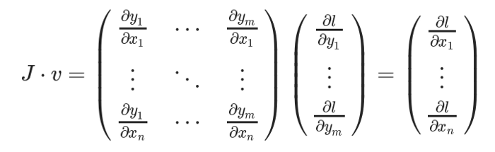
This method calculates the Jacobian matrix and compares it with the vector v The method of multiplication makes PyTorch It can easily provide external gradients for non scalar output .

The good news ！

Xiaobai learns visual knowledge about the planet

Open to the outside world

 download 1：OpenCV-Contrib Chinese version of extension module 

 stay 「 Xiaobai studies vision 」 Official account back office reply ： Extension module Chinese course , You can download the first copy of the whole network OpenCV Extension module tutorial Chinese version , Cover expansion module installation 、SFM Algorithm 、 Stereo vision 、 Target tracking 、 Biological vision 、 Super resolution processing and other more than 20 chapters .


 download 2：Python Visual combat project 52 speak 
 stay 「 Xiaobai studies vision 」 Official account back office reply ：Python Visual combat project , You can download, including image segmentation 、 Mask detection 、 Lane line detection 、 Vehicle count 、 Add Eyeliner 、 License plate recognition 、 Character recognition 、 Emotional tests 、 Text content extraction 、 Face recognition, etc 31 A visual combat project , Help fast school computer vision .


 download 3：OpenCV Actual project 20 speak 
 stay 「 Xiaobai studies vision 」 Official account back office reply ：OpenCV Actual project 20 speak , You can download the 20 Based on OpenCV Realization 20 A real project , Realization OpenCV Learn advanced .


 Communication group 

 Welcome to join the official account reader group to communicate with your colleagues , There are SLAM、 3 d visual 、 sensor 、 Autopilot 、 Computational photography 、 testing 、 Division 、 distinguish 、 Medical imaging 、GAN、 Wechat groups such as algorithm competition （ It will be subdivided gradually in the future ）, Please scan the following micro signal clustering , remarks ：” nickname + School / company + Research direction “, for example ：” Zhang San  +  Shanghai Jiaotong University  +  Vision SLAM“. Please note... According to the format , Otherwise, it will not pass . After successful addition, they will be invited to relevant wechat groups according to the research direction . Please do not send ads in the group , Or you'll be invited out , Thanks for your understanding ~