Mathematical modeling - Differential Equations

Catalog

Symbolic solutions of ordinary differential equations

Numerical solutions of ordinary differential equations

The initial value problem

The boundary value problem

  other

---

Symbolic solutions of ordinary differential equations

 diff( function ,n)% Functional n Derivative,

dsolve( equation 1, equation 2,..., equation n, Initial conditions , The independent variables )

simplify(s) For expressions s To simplify

clc,clear
syms y(x);
dy = diff(y);
s1 = dsolve((1-x)*diff(y,2)==sqrt(1+dy^2)/5,y(0)==0,dy(0)==0,x)
simplify(s1)

clc,clear
syms y(x);
out = dsolve(diff(y)==-2*y+2*x^2+2*x,y(0)==1)

clc,clear
syms y(t);% It also states that y and t
dy=diff(y);d2y=diff(y,2);d3y=diff(y,3);% The derivative is defined for the following magnitude 
u =exp(-t)*cos(t);
y = dsolve(diff(y,4)+10*diff(y,3)+35*diff(y,2)+50*diff(y)+...
    24*y==diff(u,2),y(0)==0,dy(0)==-1,d2y(0)==1,d3y(0)==1)

clc,clear
syms x(t) [3,1];% Define symbolic vector functions ,x(t) There should be a space after 
A = [3,-1,1;2,0,-1;1,-1,2];% Define coefficient matrix 
[s1,s2,s3]=dsolve(diff(x)==A*x,x(0)==[1;1;1])

Numerical solutions of ordinary differential equations

The initial value problem

A general scheme for initial value problems of first order differential equations ：

Commonly used ode45 To solve the , There are two call formats

 fun It's an anonymous function ,tspan=[t0,tfinal] Is to solve the interval ,y0 Is the initial value ,t、y Is the corresponding point of the interval and the function value of this point ,s It's an array of structures .tspan Of t0 It must be the value of the independent variable in the initial condition ,tfinal Comparable t0 Small . Utilization function deval You can calculate the function value of any point in the interval ：

y = deval(s,x);

  Example ：

clc,clear,close all
syms y(x);
% Find the symbolic solution 
y = dsolve(diff(y)==-2*y+2*x^2+2*x,y(0)==1)
% Find the numerical solution 
dy = @(x,y)-2*y+2*x^2+2*x;% The first anonymous function should be an argument , The second is the dependent variable 
[sx,sy]=ode45(dy,[0,0.5],1);    
fplot(y,[0,0.5])% Draw the image of symbolic solution 
hold on 
plot(sx,sy,'*')% Draw the image of numerical solution 
legend(' Symbolic solution ',' Numerical solution ')

matlab Higher order differential equations cannot be solved , It must be reduced to a system of first-order differential equations

Example ：

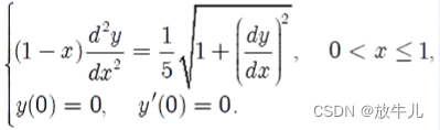
It should first be reduced to a system of first-order differential equations ：

clc,clear,close all
dy = @(x,y)[y(2);sqrt(1+y(2)^2)/5/(1-x)];
[x,y]=ode45(dy,[0,0.999999],[0;0]);
plot(x,y(:,1))

clc,clear,close all
m = 2;
df = @(x,f,m)[f(2);m*f(2)-f(1)+exp(x)];% Notice the column vector 
s1 = ode45(@(x,f)df(x,f,m),[0,1],[1;-1]);
s2 = ode45(@(x,f)df(x,f,m),[0,-1],[1;-1]);
fplot(@(x)deval(s1,x,1),[0,1],'-ok');hold on
fplot(@(x)deval(s2,x,1),[-1,0],'-*k');

  Only one order can be obtained , So define two unknowns ,ode45 The initial value of the parameter must be the function value corresponding to the left end value of the second parameter , The initial value corresponds to the horizontal axis 0, So the coordinate range is decomposed into [0,-1],[0,1]. Anonymous functions can have three parameters , but ode45 The anonymous function needs to be redefined in the function , There can only be two formal parameters .

The boundary value problem

The independent variable of the specified solution condition of the initial value problem is the same point

  The independent variable of the specified solution condition of the boundary value problem is multiple points

  The standard form of differential equation of this problem ：

 

 bc Refers to boundary conditions , The value of the independent variable in the boundary condition is also the interval of the solution , That is, the solution interval is [a,b],p Value related parameters

Correlation function ：

sol = bvp4c(odefun,bcfun,solinit,options,p1,p2,…)

odefun Functions are function handles of differential equations .bcfun The function is the handle of the boundary condition of the differential equation , Move all terms of the boundary condition to the left , On the right is 0.solinit Is the structure containing the initial estimated solution , You should use bvpinit Function creation ,solinit=bvpinit(x,y),x The vector is the sorting node of the initial mesh , The boundary conditions shall be met a= solinit.x(1) And b =solinit.x(end), vector y Is the initial estimation solution ,solinit.y(:,i) For in solinit.x(i) The initial estimation solution at the node . Output parameters sol  Is a structure containing numerical solutions ：

  To make the curve smoother , You need to insert some points in the middle , have access to deval function .

Example ：

  To a system of first order differential equations ：

  As an initial guess , You can take it

clc,clear,close all
solinit = bvpinit(linspace(-1,1,20),@dropinit);
sol = bvp4c(@drop,@dropbc,solinit)
fill(sol.x,sol.y(1,:),[0.7 0.7 0.7]);
axis([-1 1 0 1]);

function yprime = drop(x,y) % Differential equations 
yprime = [y(2),(y(1)-1)*(1+y(2)^2)^(3/2)];end

function res = dropbc(ya,yb)% The boundary conditions 
res = [ya(1);yb(1)];end     %y(1) Express y Of 0 Step derivation ,y(2) Represents the first derivative ,ya Represents the left boundary , intend ya(1)=0

function yinit = dropinit(x)% Guessing function 
yinit = [x.^2,2*x];end

  Example ：

  To a system of first order differential equations ：

 

clc,clear
eq = @(x,y,mu)[y(2),-mu*y(1)];% First order equations 
bd = @(ya,yb,mu)[ya(1);ya(2)-1;yb(1)+yb(2)];% The boundary conditions 
guess = @(x)[sin(2*x);2*cos(2*x)];% Guessing solution  
guess_structure = bvpinit(linspace(0,1,10),guess,5);
sol = bvp4c(eq,bd,guess_structure);
plot(sol.x,sol.y(1,:),'-',sol.x,sol.yp(1,:),'--')

  other

fminbnd It is used to find the minimum value of a univariate function on a definite interval