Hands on data analysis unit 3 model building and evaluation

hands-on-data-analysis Unit three Model building and evaluation

1. Model structures,

1.1. Import related libraries

import pandas as pd
import numpy as np
# matplotlib.pyplot  and  seaborn  It's a drawing library 
import matplotlib.pyplot as plt
import seaborn as sns
from IPython.display import Image

#  Embedded display picture 
%matplotlib inline

plt.rcParams['font.sans-serif'] = ['SimHei']  #  Used to display Chinese labels normally 
plt.rcParams['axes.unicode_minus'] = False  #  Used to display negative sign normally 
plt.rcParams['figure.figsize'] = (10, 6)  #  Set output picture size 

1.2. Loading of data sets

#  Read the original data set 
train = pd.read_csv('train.csv')
train.shape

Output is ：

(891, 12)

1.3. Dataset analysis

train.head()

Output is ：

	PassengerId	Survived	Pclass	Name	Sex	Age	SibSp	Parch	Ticket	Fare	Cabin	Embarked
0	1	0	3	Braund, Mr. Owen Harris	male	22.0	1	0	A/5 21171	7.2500	NaN	S
1	2	1	1	Cumings, Mrs. John Bradley (Florence Briggs Th…	female	38.0	1	0	PC 17599	71.2833	C85	C
2	3	1	3	Heikkinen, Miss. Laina	female	26.0	0	0	STON/O2. 3101282	7.9250	NaN	S
3	4	1	1	Futrelle, Mrs. Jacques Heath (Lily May Peel)	female	35.0	1	0	113803	53.1000	C123	S
4	5	0	3	Allen, Mr. William Henry	male	35.0	0	0	373450	8.0500	NaN	S

train.info()

<class 'pandas.core.frame.DataFrame'>
RangeIndex: 891 entries, 0 to 890
Data columns (total 12 columns):
 # Column Non-Null Count Dtype 
---  ------       --------------  -----  
 0   PassengerId  891 non-null    int64  
 1   Survived     891 non-null    int64  
 2   Pclass       891 non-null    int64  
 3   Name         891 non-null    object 
 4   Sex          891 non-null    object 
 5   Age          714 non-null    float64
 6   SibSp        891 non-null    int64  
 7   Parch        891 non-null    int64  
 8   Ticket       891 non-null    object 
 9   Fare         891 non-null    float64
 10  Cabin        204 non-null    object 
 11  Embarked     889 non-null    object 
dtypes: float64(2), int64(5), object(5)
memory usage: 83.7+ KB

You can see that these data still need to be cleaned , The cleaned data sets are as follows ：

# Read the cleaned data set 
data = pd.read_csv('clear_data.csv')

data.head()

	PassengerId	Pclass	Age	SibSp	Parch	Fare	Sex_female	Sex_male	Embarked_C	Embarked_Q	Embarked_S
0	0	3	22.0	1	0	7.2500	0	1	0	0	1
1	1	1	38.0	1	0	71.2833	1	0	1	0	0
2	2	3	26.0	0	0	7.9250	1	0	0	0	1
3	3	1	35.0	1	0	53.1000	1	0	0	0	1
4	4	3	35.0	0	0	8.0500	0	1	0	0	1

data.info()

Output is ：

<class 'pandas.core.frame.DataFrame'>
RangeIndex: 891 entries, 0 to 890
Data columns (total 11 columns):
 # Column Non-Null Count Dtype 
---  ------       --------------  -----  
 0   PassengerId  891 non-null    int64  
 1   Pclass       891 non-null    int64  
 2   Age          891 non-null    float64
 3   SibSp        891 non-null    int64  
 4   Parch        891 non-null    int64  
 5   Fare         891 non-null    float64
 6   Sex_female   891 non-null    int64  
 7   Sex_male     891 non-null    int64  
 8   Embarked_C   891 non-null    int64  
 9   Embarked_Q   891 non-null    int64  
 10  Embarked_S   891 non-null    int64  
dtypes: float64(2), int64(9)
memory usage: 76.7 KB

1.4. Model structures,

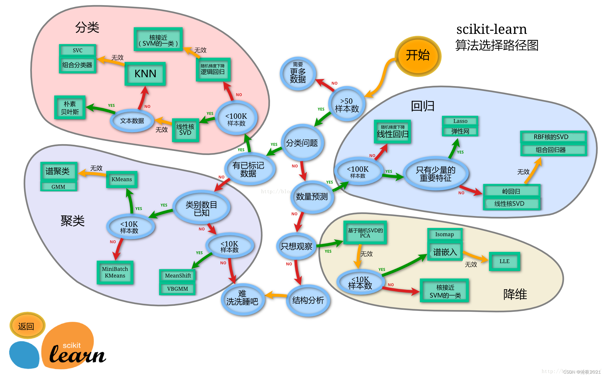
sklearn The algorithm chooses the path

Split the dataset

# train_test_split  Is a function used to cut data sets 
from sklearn.model_selection import train_test_split

#  Usually take it out first X and y Then cut , In some cases, uncut... Will be used , Now X and y You can use it ,x It's cleaned data ,y Is the survival data we want to predict 'Survived'
X = data
y = train['Survived']

#  Cut the dataset 
X_train, X_test, y_train, y_test = train_test_split(X, y, stratify=y, random_state=0)

#  View data shapes 
X_train.shape, X_test.shape

Output is ：

((668, 11), (223, 11))

X_train.info()

Output is ：

<class 'pandas.core.frame.DataFrame'>
Int64Index: 668 entries, 671 to 80
Data columns (total 11 columns):
 # Column Non-Null Count Dtype 
---  ------       --------------  -----  
 0   PassengerId  668 non-null    int64  
 1   Pclass       668 non-null    int64  
 2   Age          668 non-null    float64
 3   SibSp        668 non-null    int64  
 4   Parch        668 non-null    int64  
 5   Fare         668 non-null    float64
 6   Sex_female   668 non-null    int64  
 7   Sex_male     668 non-null    int64  
 8   Embarked_C   668 non-null    int64  
 9   Embarked_Q   668 non-null    int64  
 10  Embarked_S   668 non-null    int64  
dtypes: float64(2), int64(9)
memory usage: 82.6 KB

X_test.info()

Output is ：

<class 'pandas.core.frame.DataFrame'>
Int64Index: 223 entries, 288 to 633
Data columns (total 11 columns):
 # Column Non-Null Count Dtype 
---  ------       --------------  -----  
 0   PassengerId  223 non-null    int64  
 1   Pclass       223 non-null    int64  
 2   Age          223 non-null    float64
 3   SibSp        223 non-null    int64  
 4   Parch        223 non-null    int64  
 5   Fare         223 non-null    float64
 6   Sex_female   223 non-null    int64  
 7   Sex_male     223 non-null    int64  
 8   Embarked_C   223 non-null    int64  
 9   Embarked_Q   223 non-null    int64  
 10  Embarked_S   223 non-null    int64  
dtypes: float64(2), int64(9)
memory usage: 30.9 KB

1.5. Import model

1.5.1. Logistic regression model with default parameters

from sklearn.linear_model import LogisticRegression
from sklearn.ensemble import RandomForestClassifier

lr = LogisticRegression()
lr.fit(X_train, y_train)

Output is ：

LogisticRegression(C=1.0, class_weight=None, dual=False, fit_intercept=True,
                   intercept_scaling=1, l1_ratio=None, max_iter=100,
                   multi_class='auto', n_jobs=None, penalty='l2',
                   random_state=None, solver='lbfgs', tol=0.0001, verbose=0,
                   warm_start=False)

#  View training sets and test sets score value 
print("Training set score: {:.2f}".format(lr.score(X_train, y_train)))
print("Testing set score: {:.2f}".format(lr.score(X_test, y_test)))

Training set score: 0.80
Testing set score: 0.79

1.5.2. A logistic regression model for adjusting parameters

lr2 = LogisticRegression(C=100)
lr2.fit(X_train, y_train)

Output is ：

LogisticRegression(C=100, class_weight=None, dual=False, fit_intercept=True,
                   intercept_scaling=1, l1_ratio=None, max_iter=100,
                   multi_class='auto', n_jobs=None, penalty='l2',
                   random_state=None, solver='lbfgs', tol=0.0001, verbose=0,
                   warm_start=False)

print("Training set score: {:.2f}".format(lr2.score(X_train, y_train)))
print("Testing set score: {:.2f}".format(lr2.score(X_test, y_test)))

Output is ：

Training set score: 0.79
Testing set score: 0.78

1.5.3. Random forest classification model with default parameters

rfc = RandomForestClassifier()
rfc.fit(X_train, y_train)

Output is ：

RandomForestClassifier(bootstrap=True, ccp_alpha=0.0, class_weight=None,
                       criterion='gini', max_depth=None, max_features='auto',
                       max_leaf_nodes=None, max_samples=None,
                       min_impurity_decrease=0.0, min_impurity_split=None,
                       min_samples_leaf=1, min_samples_split=2,
                       min_weight_fraction_leaf=0.0, n_estimators=100,
                       n_jobs=None, oob_score=False, random_state=None,
                       verbose=0, warm_start=False)

print("Training set score: {:.2f}".format(rfc.score(X_train, y_train)))
print("Testing set score: {:.2f}".format(rfc.score(X_test, y_test)))

Output is ：

Training set score: 1.00
Testing set score: 0.82

1.5.4. A stochastic forest classification model with adjusted parameters

rfc2 = RandomForestClassifier(n_estimators=100, max_depth=5)
rfc2.fit(X_train, y_train)

Output is ：

RandomForestClassifier(bootstrap=True, ccp_alpha=0.0, class_weight=None,
                       criterion='gini', max_depth=5, max_features='auto',
                       max_leaf_nodes=None, max_samples=None,
                       min_impurity_decrease=0.0, min_impurity_split=None,
                       min_samples_leaf=1, min_samples_split=2,
                       min_weight_fraction_leaf=0.0, n_estimators=100,
                       n_jobs=None, oob_score=False, random_state=None,
                       verbose=0, warm_start=False)

print("Training set score: {:.2f}".format(rfc2.score(X_train, y_train)))
print("Testing set score: {:.2f}".format(rfc2.score(X_test, y_test)))

Output is ：

Training set score: 0.87
Testing set score: 0.81

1.6. prediction model

General supervisory model in sklearn There's a predict Can output prediction labels ,predict_proba Label probability can be output

#  Forecast tags 
pred = lr.predict(X_train)

#  Now we can see 0 and 1 Array of 
pred[:10]

Output is ：

array([0, 1, 1, 1, 0, 0, 1, 0, 1, 1])

#  Predicted tag probability 
pred_proba = lr.predict_proba(X_train)

pred_proba[:10]

Output is ：

array([[0.60884602, 0.39115398],
       [0.17563455, 0.82436545],
       [0.40454114, 0.59545886],
       [0.1884778 , 0.8115222 ],
       [0.88013064, 0.11986936],
       [0.91411123, 0.08588877],
       [0.13260197, 0.86739803],
       [0.90571178, 0.09428822],
       [0.05273217, 0.94726783],
       [0.10924951, 0.89075049]])

2. Model to evaluate

2.1. Cross validation

There are many kinds of cross validation , The first is the simplest , It's easy to think of ： Divide the data set into two parts , Is a training set （training set）, One is the test set （test set）.

however , There are two drawbacks to this simple approach .

1. The final model and parameter selection will largely depend on how you divide the training set and test set .

2. This method only uses part of the data to train the model , Failure to take full advantage of the data in the dataset .

To solve this problem , The following technicians have carried out a variety of optimizations , The next step is K Crossover verification ：

We will no longer have only one data per test set , It's more than one. , The specific number will be based on K The choice of . such as , If K=5, So the steps we take to cross verify with a 30% discount are ：

1. Divide all data sets into 7 Share

2. Do not repeatedly take one of them at a time as a test set , Use other 6 Make a training set training model , And then calculate the MSE

3. take 7 Take the average of times to get the final MSE

from sklearn.model_selection import cross_val_score

lr = LogisticRegression(C=100)
scores = cross_val_score(lr, X_train, y_train, cv=10)

# k Fold cross validation score 
scores

Output :

array([0.82089552, 0.74626866, 0.74626866, 0.7761194 , 0.88059701,
       0.8358209 , 0.76119403, 0.8358209 , 0.74242424, 0.75757576])

#  Average cross validation score 
print("Average cross-validation score: {:.2f}".format(scores.mean()))

Output ：

Average cross-validation score: 0.79

2.2. Confusion matrix

Confusion matrix is used to summarize the results of a classifier . about k Metaclassification , In fact, it is a k x k Table for , Used to record the prediction results of the classifier .

The method of confusion matrix is sklearn Medium sklearn.metrics modular

The confusion matrix needs to input the real label and prediction label

Accuracy 、 Recall rate and f- Scores can be used classification_report modular

In fact, the quality of the model , Just look at the main diagonal of the confusion matrix .

from sklearn.metrics import confusion_matrix

#  Training models 
lr = LogisticRegression(C=100)
lr.fit(X_train, y_train)

LogisticRegression(C=100, class_weight=None, dual=False, fit_intercept=True,
                   intercept_scaling=1, l1_ratio=None, max_iter=100,
                   multi_class='auto', n_jobs=None, penalty='l2',
                   random_state=None, solver='lbfgs', tol=0.0001, verbose=0,
                   warm_start=False)

#  Model predictions 
pred = lr.predict(X_train)

#  Confusion matrix 
confusion_matrix(y_train, pred)

array([[354,  58],
       [ 83, 173]])

#  Classified reports 
from sklearn.metrics import classification_report

#  Accuracy 、 Recall rate and f1-score
print(classification_report(y_train, pred))

    			precision    recall  f1-score   support

           0       0.81      0.86      0.83       412
           1       0.75      0.68      0.71       256

    accuracy                           0.79       668
   macro avg       0.78      0.77      0.77       668
weighted avg       0.79      0.79      0.79       668

2.3.ROC curve

ROC The curve originated from the judgment of radar signal by radar soldiers during World War II . At that time, the task of every radar soldier was to analyze the radar signal , But the radar technology was not so advanced at that time , There is a lot of noise , So whenever a signal appears on the radar screen , Radar soldiers need to decipher it . Some radar soldiers are more cautious , Whenever there is a signal , He tends to interpret it as an enemy bomber , Some radar soldiers are more nervous , It tends to be interpreted as a bird . In this case, a set of evaluation indicators is urgently needed to help him summarize the prediction information of each radar soldier and evaluate the reliability of this radar . therefore , One of the earliest ROC The curve analysis method was born . After that ,ROC Curve is widely used in medicine and machine learning .

ROC The full name is Receiver Operating Characteristic Curve, The Chinese name is 【 The working characteristic curve of subjects 】

ROC The curve is in sklearn The module in is sklearn.metrics

ROC The larger the area surrounded by the curve, the better

from sklearn.metrics import roc_curve

fpr, tpr, thresholds = roc_curve(y_test, lr.decision_function(X_test))
plt.plot(fpr, tpr, label="ROC Curve")
plt.xlabel("FPR")
plt.ylabel("TPR (recall)")
#  Find the closest to 0 The threshold of 
close_zero = np.argmin(np.abs(thresholds))
plt.plot(fpr[close_zero], tpr[close_zero], 'o', markersize=10, label="threshold zero", fillstyle="none", c='k', mew=2)
plt.legend(loc=4)

3. Reference material

【 machine learning 】Cross-Validation（ Cross validation ） Detailed explanation - You know (zhihu.com)

https://www.jianshu.com/p/2ca96fce7e81