Statistical machine learning code set

P39 Exercise application 8

college = read.csv("./data/College.csv",sep = ',',header = TRUE);


rownames(college) = college[,1] #  Make the first column row name 
# fix(college)
college = college[,-1]  #  Delete the first column 
# fix(college)

college$Private=huaas.factor(college$Private)  # Private Is a character variable   So factorization 

#  Data characteristics 
summary(college)

#  Scatter matrix 
pairs(college)

#  boxplot 
plot(college$Private, college$Outstate)  # P Yes O Along the side of the box line diagram 
   #  Abscissa for P Of Yes and NO , Ordinate for O The numerical 

Elite = rep("No", nrow(college))  #  Create a list Elite, Duplicate assignment college Number of lines No
Elite[college$Top10perc>50]="Yes"   #  Greater than 50 assignment Y  Vector operations 
Elite = as.factor(Elite)  #  Into factors 
college = data.frame(college, Elite) #  Merge 
summary(Elite)
plot(college$Elite, college$Outstate)


#  Histogram 
par(mfrow = c(2,2)) #  Window partition 
hist(college$Accept,breaks = 5, prob=T)
hist(college$Accept,breaks = 10, prob=T)
hist(college$Accept,breaks = 20, prob=T)
hist(college$Accept,breaks = 50, prob=T)

The second assignment

1. Artificial data : Generate 200 individual f(x)=sinx y=f(x)+ei~N(0,0.2) Generate a normal distribution random number rnorm
2. Linear regression fitting data ： Output mean square error
3. Polynomial function poly（1,3,5,20,23） Fit points again

#  Generate sin+ Noise data 
set.seed(11)  #  Set random seeds 
x = runif(200,-10,10); # 200 individual -10 To 10 A random number evenly distributed between 
x = sort(x)  #  Sort 
y = sin(x)+rnorm(200,0,0.2)   # sinx+e,e The mean value of the normal distribution is 0, The variance of 0.2 Random disturbance of 

#  drawing 
plot(x,y,type = 'l',col = 'red',main = "Ganerate random data")
lines(x,sin(x),col = 'blue')
legend(x = 'bottomleft', 
       legend = c(expression(y == sinx+e), expression(y == sinx)),
       lty =1,
       col = c('red', 'blue'),
       bty = 'n',
       horiz = T,
       cex = 0.8)
       
#  Calculation mse function 
MSE_fit = function(y,fit,p){
    
  n=length(fit$residuals)
  rse = sqrt(sum(fit$residuals^2)/(n-p-1)) # https://www.cnblogs.com/HuZihu/p/9692814.html
  mse1 = rse^2*((n-p-1)/n);mse1
}

#  Linear regression 
fit1 = lm(y~x)
summary(fit1)
MSE_fit(y,fit1,1)  #  Calculation mse

#  Make a comparison 
plot(x,y,main = "Linear regression",cex = 0.8)
fit1_y = predict(fit1)
lines(x,fit1_y,col ='red')
legend(x = 'bottomleft', 
       legend = c(expression(y == sinx+e), expression('Predicts')),
       lty =1,
       col = c('black', 'red'),
       bty = 'n',
       horiz = T,
       cex = 0.8)

#  Polynomial plot legend function 
pr_plot = function(x,y,fit,main_num){
    
  plot(x,y,main = main_num, cex = 0.8)
  fit_y = predict(fit)
  lines(x,fit_y, col = 'red')
  legend(x = 'bottomleft', 
        legend = c(expression(y == sinx+e), expression('Predicts')),
        lty =1,
        col = c('black', 'red'),
        bty = 'n',
        horiz = T,
        cex = 0.8)
        
#  Polynomial function fitting 
#  Method 1 ： Draw a picture each 
mse = c()
for(i in seq(3,14)){
    
  fit = lm(y~poly(x, i))  #  Polynomial function 
  pr_plot(x,y,fit,paste('Polynomial regression',i))
  mse = c(mse,MSE_fit(fit, i))
}
mse
}

#  Method 2 ： The line is drawn on a diagram 
mse = c()
plot(x,y)
for(i in seq(3,14)){
    
  fit = lm(y~poly(x, i))
  mse = c(mse,MSE_fit(fit, i))
  lines(x,predict(fit),col=i)  
}
mse

# Simulated data  Generate the data 
GenerateDataSin = function(n, sigma1, sigma2)
{
    
  x = seq(0,2*pi,length.out = n)  # x Range and output length n
  set.seed(1) #  Set random seeds 
  r = rnorm(n, mean = 0, sd = sigma1) # x Random disturbance of   To obey the mean is 0, The variance of sigma1 Is a normal distribution 
  X = x + r
  set.seed(2)  
  epsilon = rnorm(n, mean = 0, sd = sigma2)  #  Random error term 
  Y = sin(X) + epsilon 
  dataAll = data.frame(X,Y) # x y  Merge into data frame 
  return(dataAll)  #  Return to the data box 
}

# Getting training and test data  Generating training sets and test sets 
TrainData = GenerateDataSin(60, 0.1, 0.3)  #  Training set 
par(mfrow = c(1, 2))
plot(TrainData$X, TrainData$Y, xlab = "X", ylab = "Y")
TestData = GenerateDataSin(30, 0.1, 0.3)  #  Test set 
points(TestData$X, TestData$Y,col = "green") #  Test set points "Green" points represent the test data

#  Standard image rendering 
xx = seq(0,2*pi, by = 0.1)   # 0 To 2pi, The interval is 0.1
lines(xx,sin(xx))  # sinx Standard image 


# Fitting the model  Fitting model 
ModelSin = function(Train, Test, k) # k Is the degree of a polynomial 
{
    
  modelfit.lm = lm(Y~poly(X, k), data = Train)  #  Linear regression 
  trainX = Train$X
  tstX = Test$X
  yhat.train = predict(modelfit.lm, data.frame(X = trainX))  #  Prediction on the training set 
  yhat.tst = predict(modelfit.lm, data.frame(X = tstX))  #  Test set prediction 
  lines(trainX, yhat.train, col = k) #  Training set fitting line 
  trainMSE = mean((Train$Y - yhat.train)^2)  #  Training mse  Mean square error of training set 
  tstMSE = mean((Test$Y - yhat.tst)^2)   #  Mean square error of test set 
  Output = list(yhat.tst,trainMSE,tstMSE)  #  Returns the test set prediction   Training mean square error   Test mean square error 
  return(Output)
}

Output1 = ModelSin(TrainData, TestData, 1) #  once   Simple linear regression 
Output3 = ModelSin(TrainData, TestData, 3) #  Green curve 
Output20 = ModelSin(TrainData, TestData, 20)  #  Blue 
Output23 = ModelSin(TrainData, TestData, 23)  #  yellow 

# MSE
TrainMSE = c(Output1[[2]], Output3[[2]], Output20[[2]], Output23[[2]])
TrainMSE  #  Mean square error of training set   With the increase of smoothness   Monotonic decline 
TestMSE = c(Output1[[3]], Output3[[3]], Output20[[3]], Output23[[3]])
TestMSE  #  Mean square error of test set   As the smoothness increases u Shape distribution 
plot(TestMSE,xlab = "Complexity of model", ylab = "MSE")
lines(TestMSE, col = "red")
points(TrainMSE)
lines(TrainMSE, col = "grey")

The third chapter Simple linear regression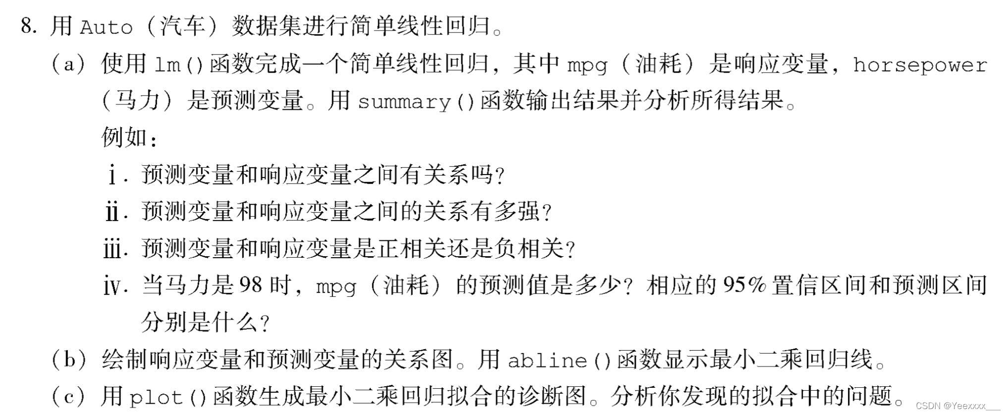

Auto = read.csv("./data/Auto.csv")
for(i in 1:length(Auto[,1])){
    
  if(Auto$horsepower[i] == "?"){
    
    Auto$horsepower[i] = NA
  }
}   #  In the data ？ To deal with 
Auto = na.omit(Auto)  #  Delete null 
class(Auto$horsepower)  # "character"
Auto$horsepower = as.numeric(Auto$horsepower) #  The conversion type is numeric 
attach(Auto)


# lm  Simple linear regression  
  #  Whether there is a correlation between the two 
cor.test(mpg,horsepower)
  # Pearson's product-moment correlation
  # 
  # data: mpg and horsepower
  # t = -24.489, df = 390, p-value < 2.2e-16
  # alternative hypothesis: true correlation is not equal to 0
  # 95 percent confidence interval:
  # -0.8146631 -0.7361359
  # sample estimates:
  # cor 
  # -0.7784268 
    #  Judging from the correlation coefficient ,mpg And horsepower Has a highly negative correlation , The correlation coefficient is as high as 0.778
    #  Further, we can test the significance of correlation ,
    # H0 by X and Y There is no correlation between ,p Far less than 0.05, Rejection of null hypothesis , There must be a relationship between the two .
    
fit1 = lm(mpg~horsepower) #  Fitting a simple linear regression model  
summary(fit1)  #  Details 
coef(fit1)  #  Parameters 
  #  The model is written in equation form  ：mpg = 39.9358610 - 0.1578447 * horsepower 
#  When horsepower=98 The predicted value is ?
a = as.data.frame(98)
colnames(a)=list("horsepower") 
predict(fit1,a)  # 24.46708 
#  When horsepower=98 when   The corresponding confidence interval is ？[23.97308 24.96108]
predict(fit1,a,interval = "confidence")
  # fit lwr upr
  # 1 24.46708 23.97308 24.96108
  #  Predictive value   Lower confidence interval / ceiling 
#  When horsepower=98 when   The corresponding prediction interval is ？[14.8094 34.12476]
predict(fit1,a, interval = "prediction")
  # fit lwr upr
  # 1 24.46708 14.8094 34.12476

#  Plot the relationship between response variables and prediction variables , use abline() The function shows the least squares regression line 
plot(horsepower,mpg,col="red") 
abline(fit1,col="blue",lw=2)

#  Regression diagnosis diagram 
par(mfrow = c(2, 2))
plot(fit1)
	# Residuals vs Fitted： The relationship between residuals and estimates , The data points should be roughly twice the standard deviation, that is 2、-2 And   between , And these points should not show any regular trend .
	# Normal QQ： If the normal hypothesis is satisfied , So the points on the graph should fall on the 45 On the line of the degree Angle ; If not , Then it violates the assumption of normality .
	# Scale-Location：GM The homovariance in the hypothesis can be diagnosed by this graph , The variance should be basically fixed or flat .
	# Cook’s distance：Cook distance , For diagnosis of strong influence points .

Auto$name = as.factor(name) #  Into factors 
pairs(Auto)  #  Draw a matrix scatter 
#  Calculate the correlation coefficient matrix between variables , Exclude qualitative variables name
cor(Auto[,1:8])
  
  #  Multiple linear regression 
fit2 = lm(mpg~.-name,data = Auto) 
summary(fit2)
  #（1） from F The statistical value is 254.4 You know , Far greater than  1, And  F  Statistical  p  The value is almost zero .  Explain that at least one prediction variable is related to the response variable .
  #（2） From the model information , Predictive variables displacement、weight、year、origin Of  p  Less value , It has a significant relationship with the response variables . 
  #（3）year  The coefficient of is positive , It means that with the increase of vehicle age , Fuel consumption will increase . Increase the vehicle age by one year , The average mileage per barrel of oil has increased 0.7508 km 
par(mfrow=c(2,2)) 
plot(fit2)

  #  Linear regression model fitting with interactive terms 
fit3 = lm(mpg~.-name+horsepower*cylinders,data=Auto) 
summary(fit3)
  #  There are statistically significant interactions , But the coefficient is small .
  
  #  Nonlinear transformation 
fit4 = lm(mpg ~ .-name + log(horsepower), data=Auto)
summary(fit4)
  # horsepower  Logarithmic term of  p  The value is almost  0, It shows that there is a nonlinear relationship between some prediction variables and response variables .

fit5 = lm(mpg ~ .-name + sqrt(horsepower), data=Auto) #  Open the root 
summary(fit5)

The fifth chapter Resampling method

### (a) Generate an analog data set as follows ：
set.seed(1)
y=rnorm(100)
x=rnorm(100)
y=x-2*x^2+rnorm(100)
	# n = 100, p = 2. 
	#  The model form is  $Y=X−2X^2+ϵ$.

### (b) do X Yes Y The scatter diagram of 
plot(x, y)

### (c)LOOCV error 
library(boot)
data = data.frame(x, y)  #  Define the data frame 
	#  function ： Leave one way to fit + Return error 
Loocv_fit = function(seed,po){
      # po（poly）
  set.seed(seed)
  glm.fit = glm(y ~ poly(x, po))  #  Fitting model  glm and lm equally , It's just glm You can talk to cv.glm Together with 
  cv.err = cv.glm(data, glm.fit) #  The first parameter is data   The second parameter is the model 
  return(cv.err$delta)  #  Results of cross validation ： The original result   And adjusted results 
}

for(i in 1:4){
    
  print(i)
  print(Loocv_fit(11,i)) # 11 It's a random seed 
}
#  The selected model is quadratic by cross validation 

### (d)  Transform random seeds 
for(i in 1:4){
    
  print(i)
  print(Loocv_fit(12,i))
}
# The results have not changed , because LOOCV There is no randomness in the segmentation between the training set and the verification set , So you always get the same result 

### （e）
# ii. $Y= \beta_{0} + \beta_{1}X + \beta_{2}X^2 + ϵ$  There is the smallest LOOCV error , Consistent with the expected results , because （a） The form of the model that generates random numbers in is quadratic , It shows that we can pass LOOCV Choose a better model .

### （f） see t Check whether the selected features are consistent with the results of cross validation 
fit = glm(y ~ poly(x, 4))
summary(fit)
#  Agreement , Of primary and secondary terms p Less than 0.05, Statistically significant , Three times and four times are not significant . The results of statistical tests are consistent with LOOCV Consistent result .

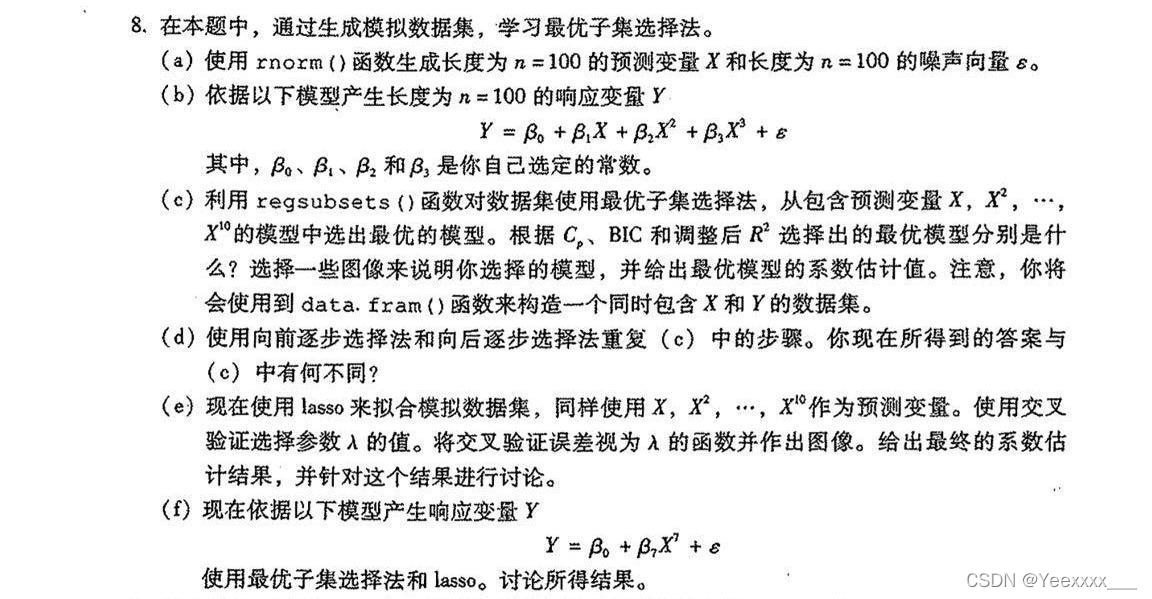
# P182 8 abcd
### (a) Generate x  and  $\epsilon$ 
set.seed(1) #  Set random seeds 
X = rnorm(100)
eps = rnorm(100)

### (b)  Build a model , Generate response variables Y
beta0 = 1
beta1 = 3
beta2 = -2
beta3 = 0.5
Y = beta0 + beta1 * X + beta2 * X^2 + beta3 * X^3 + eps

library(leaps)
data = data.frame(y = Y, x = X)  #  The construct also contains X and Y Data set of 、 box 
regfit.full = regsubsets(y ~ poly(x, 10, raw = T), data = data, nvmax = 10)  # ?raw  Optimal subset selection method  nvmax Is the maximum number of features selected 
mod.summary = summary(regfit.full)
mod.summary

#  adopt cp、bic、adjust R^2 Decide which model is the best ,cp bic Minimum ,adjustR^2 Maximum 
which.min(mod.summary$cp)
which.min(mod.summary$bic)
which.max(mod.summary$adjr2)
	#cp、bic Minimum ,adjust $R^2$ The biggest ones are 3

#  visualization cp
par(mfrow = c(1,2))
plot(mod.summary$cp, ylab = "Cp",type = "l")  #  Ten models cp Line chart of 
points(3, mod.summary$cp[3],col = "red", lwd = 2)
plot(regfit.full,scale = 'Cp') 
#  visualization bic
par(mfrow = c(1,2))
plot(mod.summary$bic, ylab = "BIC",type = "l")
points(3, mod.summary$bic[3],col = "red", lwd = 2)
plot(regfit.full,scale = 'bic')
#  visualization adjr2
par(mfrow = c(1,2))
plot(mod.summary$adjr2, ylab = "Adjusted R2",type = "l")
points(3, mod.summary$adjr2[3],col = "red", lwd = 2)
plot(regfit.full,scale = 'adjr2')

#  Fitting the cubic model 
b_fit=lm(y ~ poly(x,3, raw = T), data = data) 
summary(b_fit)
coef(b_fit)  #  The estimation coefficient of the optimal model   The true coefficient is  1 3 -2 0.5


### (d) Step forward and backward 
mod.fwd = regsubsets(y ~ poly(x, 10, raw = T), data = data, nvmax = 10, 
    method = "forward") #  forward 
mod.bwd = regsubsets(y ~ poly(x, 10, raw = T), data = data, nvmax = 10, 
    method = "backward")  #  backward 
fwd.summary = summary(mod.fwd)
bwd.summary = summary(mod.bwd)

which.min(fwd.summary$cp)
which.min(fwd.summary$bic)
which.max(fwd.summary$adjr2)

which.min(bwd.summary$cp)
which.min(bwd.summary$bic)
which.max(bwd.summary$adjr2)

#  And （c） The results of optimal subset selection in are consistent , Are all 3 Time , Because this experiment p Is not big , The optimal subset selection method is still applicable , Step by step forward and backward, we also get consistent results , For the time being, the forward and backward step-by-step selection method is still very good , It's very efficient , It's also more accurate .