当前位置:网站首页>Teacher Wu Enda's machine learning course notes 02 univariate linear regression
Teacher Wu Enda's machine learning course notes 02 univariate linear regression
2022-07-29 06:53:00 【three billion seventy-seven million four hundred and ninety-one】
2 Univariate linear regression
2.1 Model describes
Next, we will continue with the following content based on the example of predicting house prices mentioned in Chapter 1 .
Token Convention
In supervised learning, there is a data set , This data set is called the training set . Throughout the course m m m To represent the number of training samples .
use x x x Represents the input variable ( features ), use y y y Represents the output variable ( Target variables to be predicted ).
use ( x , y ) (x,y) (x,y) Represents a training sample , use ( x ( i ) , y ( i ) ) (x^{(i)},y^{(i)}) (x(i),y(i)) It means the first one i i i Training samples , Note the superscript i i i Not an index , It's an index of the dataset .
Supervise the working process of the learning algorithm
Provide training sets to learning algorithms , The task of learning algorithm is to output a hypothetical function , Usually use h h h Express .
Suppose that the function is to predict the output corresponding to the input .
Hypothesis function
Designing learning algorithms first requires deciding how to represent hypothetical functions h h h.
One possible expression is , h θ ( x ) = θ 0 + θ 1 x h_{\theta}(x)=\theta_{0}+\theta_{1} x hθ(x)=θ0+θ1x. This means that the next hypothetical function will predict y y y About x x x The linear function of .
Because it contains only one feature / The input variable , And it is linear , Therefore, such regression problems are called univariate linear regression problems or univariate linear regression problems .
summary
The working process of supervising learning is , By providing a training set to the learning algorithm , The learning algorithm outputs a hypothetical function h h h.
Here we will first assume the function h h h As a linear function .
2.2 Cost function
The cost function is to find the best line to fit the data .
Model parameters
For hypothetical functions h θ ( x ) = θ 0 + θ 1 x h_{\theta}(x)=\theta_{0}+\theta_{1} x hθ(x)=θ0+θ1x, θ 0 \theta_{0} θ0 and θ 1 \theta_{1} θ1 Is the model parameter .
Squared error function
Through the cost function , You can find a line that fits the data better , Thus, the model parameters that can minimize the modeling error can be obtained .
Usually we can use the square error function J ( θ 0 , θ 1 ) = 1 2 m ∑ i = 1 m ( h θ ( x ( i ) ) − y ( i ) ) 2 J\left(\theta_{0}, \theta_{1}\right)=\frac{1}{2 m} \sum_{i=1}^{m}\left(h_{\theta}\left(x^{(i)}\right)-y^{(i)}\right)^{2} J(θ0,θ1)=2m1∑i=1m(hθ(x(i))−y(i))2 As a cost function , For most problems , Especially the problem of return , The square error cost function is a reasonable choice , Of course, there are other types of cost functions .
Our optimization goal is to minimize the cost function .
summary
For hypothetical functions h θ ( x ) = θ 0 + θ 1 x h_{\theta}(x)=\theta_{0}+\theta_{1} x hθ(x)=θ0+θ1x, θ 0 \theta_{0} θ0 and θ 1 \theta_{1} θ1 Is the model parameter .
Usually, the square error function can be used as the cost function , Thus, the model parameters that can minimize the modeling error can be obtained .
2.3-2.4 An intuitive understanding of the cost function
Hypothetical function and cost function
| Hypothesis function h θ i ( x ) h_{\theta_{i}}(x) hθi(x) | Cost function J ( θ i ) J(\theta_{i}) J(θi) | |
|---|---|---|
| The independent variables | For a given θ \theta θ, h h h It's about x x x Function of | J J J It's about θ \theta θ Function of |
| Function image |  |  |
2.5-2.6 Gradient descent method
Gradient descent method
Gradient descent method is an algorithm for finding the minimum value of a function , This method can be used to minimize the cost function .
First, a combination of parameters is randomly selected to calculate the cost function , Then find the next parameter combination that can reduce the value of the cost function the most . Keep doing this until you reach a local minimum (local minimum).
Because I didn't try all the parameter combinations , Therefore, it is uncertain whether the local minimum found is the global minimum (global minimum).
Choose different combinations of initial parameters , Different local minima may be found .
The mathematical principle of gradient descent method
Repeat until convergence {
θ j : = θ j − α ∂ ∂ θ j J ( θ 0 , θ 1 ) (for j = 0 and j = 1 ) \theta_{j}:=\theta_{j}-\alpha \frac{\partial}{\partial \theta_{j}} J\left(\theta_{0}, \theta_{1}\right) \quad \text { (for } j=0 \text { and } j=1 \text { ) } θj:=θj−α∂θj∂J(θ0,θ1) (for j=0 and j=1 )
}
It should be noted that : = := := Represents the assignment operator , and = = = Indicates that the left and right values are equal .
α \alpha α It's the learning rate , It's used to control the step size when the gradient drops .
What needs to be explained is the parameter θ 0 \theta_{0} θ0 and θ 1 \theta_{1} θ1 Need to synchronize updates , That is, the right part of the calculation formula should be stored in the temporary variable , Then use temporary variables to update at the same time θ 0 \theta_{0} θ0 and θ 1 \theta_{1} θ1.
Understanding of gradient descent method
If α \alpha α Too small , It takes many steps to reach the local lowest point ; If α \alpha α Too big , May not converge .
also , With the operation of gradient descent method , The derivative value will become smaller and smaller , The range of movement will become smaller and smaller , Until it converges to the local minimum , Local best , The derivative value is 0, Therefore, there is no need to further reduce α \alpha α Value .
summary
Gradient descent method is an algorithm for finding the minimum value of a function , This method can be used to minimize the cost function .
α \alpha α It's the learning rate , It's used to control the step size when the gradient drops .
With the operation of gradient descent method , The derivative value will become smaller and smaller , The range of movement will become smaller and smaller , Until it converges to the local minimum .
2.7 The gradient of linear regression decreases
The local optimal solution of the linear regression cost function is the global optimal solution
Initializing with different values may lead to convergence to different local optimal solutions , The local optimal solution converged to may not be the global optimal solution .

But as shown above , The cost function of linear regression is convex , The local optimal solution is the global optimal solution .
Batch gradient descent method (Batch Gradient Descent)
Gradient descent method is also called batch gradient descent method (Batch Gradient Descent), It means that in every step of the gradient descent , All the training samples are used . When calculating partial derivatives , The calculation is the sum of the individual gradient descent of all training samples .
summary
Using the gradient descent method for the cost function of linear regression can converge to the global optimal solution of the function .
Gradient descent method is also called batch gradient descent method , In every step of the descent , The calculation is the sum of the individual gradient descent of all training samples .
边栏推荐
- Teacher wangshuyao's notes on operations research 06 linear programming and simplex method (geometric significance)
- How to write controller layer code gracefully?
- Invalid access control
- Hongke shares | how to test and verify complex FPGA designs (1) -- entity or block oriented simulation
- Base64与File之间的相互转化
- 【技能积累】写邮件时的常用表达
- 10 frequently asked JVM questions in interviews
- 基于噪声伪标签和对抗性学习的医学图像分割注释有效学习
- 王树尧老师运筹学课程笔记 01 导学与绪论
- CVPR2022Oral专题系列(一):低光增强
猜你喜欢

5G服务化接口和参考点

Shallow reading of condition object source code
5g service interface and reference point

SQL developer graphical window to create database (tablespace and user)

基于噪声伪标签和对抗性学习的医学图像分割注释有效学习

Joint modeling of price preference and interest preference in conversation recommendation - extensive reading of papers

Annotation
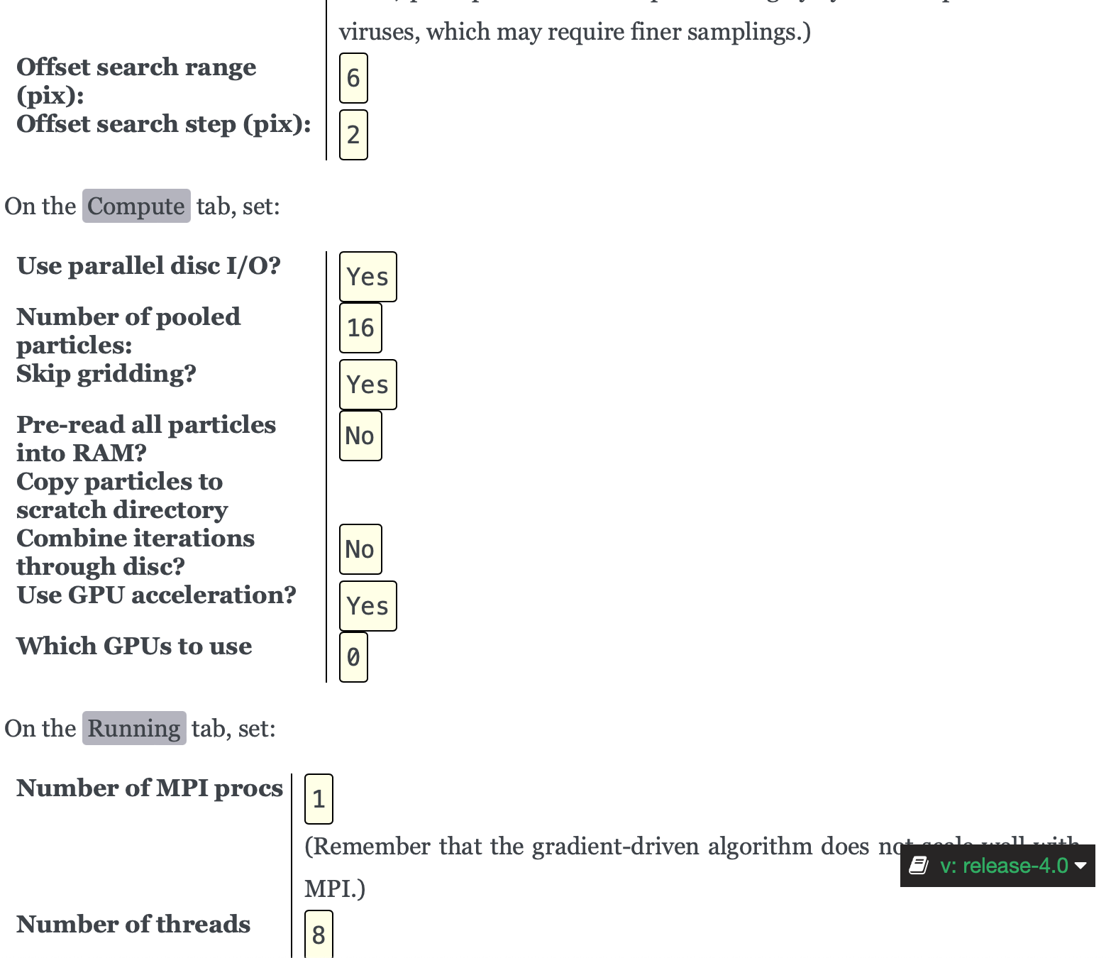
【冷冻电镜】Relion4.0——subtomogram教程

Actual combat! Talk about how to solve the deep paging problem of MySQL

CNN-卷积神经网络
随机推荐
Biased lock, lightweight lock test tool class level related commands
DBAsql面试题
模拟卷Leetcode【普通】093. 复原 IP 地址
ping 原理
Difference between CNAME record and a record
Teacher wangshuyao's notes on operations research course 08 linear programming and simplex method (simplex method)
Ping principle
二次元卡通渲染——进阶技巧
Teacher Cui Xueting's course notes on optimization theory and methods 00 are written in the front
【备忘】关于ssh为什么会失败的原因总结?下次记得来找。
Let the computer run only one program setting
5G控制面协议之N2接口
【技能积累】presentation实用技巧积累,常用句式
Share some tips for better code, smooth coding and improve efficiency
Talk about tcp/ip protocol? And the role of each layer?
【笔记】The art of research - (讲好故事和论点)
Embedding理解+代码
Phantom reference virtual reference code demonstration
崔雪婷老师最优化理论与方法课程笔记 00 写在前面
【解决方案】ERROR: lib/bridge_generated.dart:837:9: Error: The parameter ‘ptr‘ of the method ‘FlutterRustB